Machine Learning By Andew Ng - Week 1

Welcome

Machine learning is the science getting computers to learn, without explicitly programmed.

Welcome

• Many AI researchers believe that the best way towards the goal of developing AI as same intelligence as humans will be through learning algorithms that try to mimic how the human brain learns.

Machine Learning

• Grew out of work in AI

• New capability for computers

Examples :

• Database Mining

  • Large Datasets from growth of automation/web

  • E.g. Web click data, medical records, biology, engineering

• Applications can’t program by hand

  • E.g. Autonomous helicopter, handwriting recognition, most of Natural Language Processing, computer vision

• Self-customising programs

  • E.g. Amazon, Netflix product recommendations

• Understanding human learning ( brain, real AI )

What is Machine Learning ?

Definition

• Arthur Samuel ( 1959 ). Machine Learning: Field of study that gives computers the ability to learn without being explicitly programmed.

  • Checkers game

• Tom Mitchell ( 1998 ). Well-posed learning

  • Problem: A computer program is said to learn from experience E with respect to some task T and some performance measure P, if its performance on T, as measured by P, improves with experience E.

Machine Learning Algorithms:

• Supervised Learning

• Unsupervised Learning

Other: Reinforcement learning, recommender systems.

Supervised Learning

Housing Prices Prediction

• If we have a dataset of house prices and we plot it on a graph. How can we find the rate of the new house based on the size. On x-axis we plot size and on y-axis we plot price. We can draw a line between the data and calculate or we can draw a curve and then calculate.

• This is an example of Supervised Learning algorithm

  • We gave the right answers

• This can also be called as regression problem.

  • Predict continuous valued output (price)

Breast cancer (malignant, benign)

• If we want to predict which tumor is malignant and benign. First we have the dataset plotted. On x-axis the size of the tumor and on y-axis malignant.

• Feature over here is the size of the tumor.

• This is a *problem.

  • Discrete Valued Output

    • Can be more than 2 output values

• We can plot the data on a single line.

• Features can be more than one.

• Now, we have to features age and tumor size. After plotting the data we can draw a line between the section of malignant or benign.

Unsupervised Learning

• When there is a dataset with no labels or same labels and we have not told what to do with it.

• Finding the structure in the dataset is the motive.

• If the data points can be clustered. Then it is a clustering algorithm.

  • E.g. Google news clustering

    • Grouping same stories based on same news

  • Human gene

    • Which human has which gene. Clustering them using the colours.

  • Organise computing clusters

    • Running data centres efficiently

  • Social network analysis

    • Using data from different social networks, close friends can be predicted of a particular person.

  • Market segmentation

    • By having the customer data, we can predict that which customer corresponds to which marker segment.

  • Astronomical data analysis

    • By using the data, we can predict how the galaxies are formed

Cocktail Party Problem

• This is a non-clustering problem.

• In a party if there are two speakers and two microphones are placed far relatively to the speakers. Speaker 1 is clearer to the microphone 1 and less audible to the microphone 2 and vice versa.

• Each microphone records the overlapping voice of both of the speakers.

  • This both can be given to the cocktail party algorithm. This algorithm will separate out the two voices.

• Algorithm can be done in one line of code

  • [W,s,v] = svd((repmat(sum(x.x,1),size(x,1),1).x)*x’);

    • Octave programming environment

    • svd - single value decomposition

Model and Cost Function

Model Representation

• Supervised Learning - House price

• Notation

  • m = Number of training examples

  • x’s = ‘‘input’’ variable / features

  • y’s = “output” variable

  • (x,y) = one training example

  • (x^i, y^i) = i th training example

• Process Flow

  • Training Set → Learning Algorithm → h (hypothesis)

  • Hypothesis is a function given by the algorithm, which when inputed the data gives the suitable output based on the previous data.

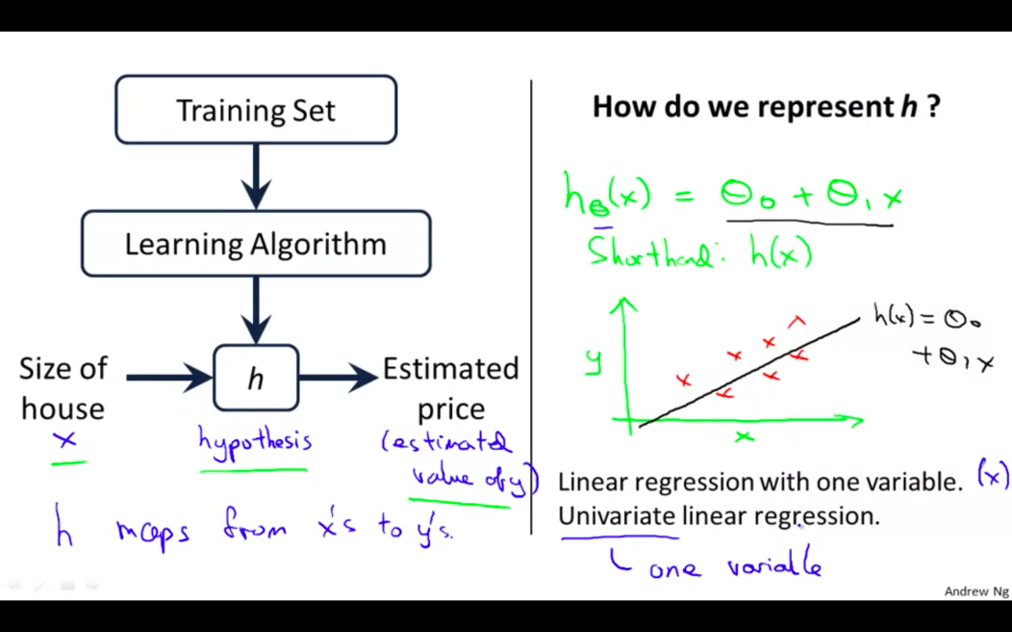
Cost Function

• Used to measure the accuracy of our hypothesis function.

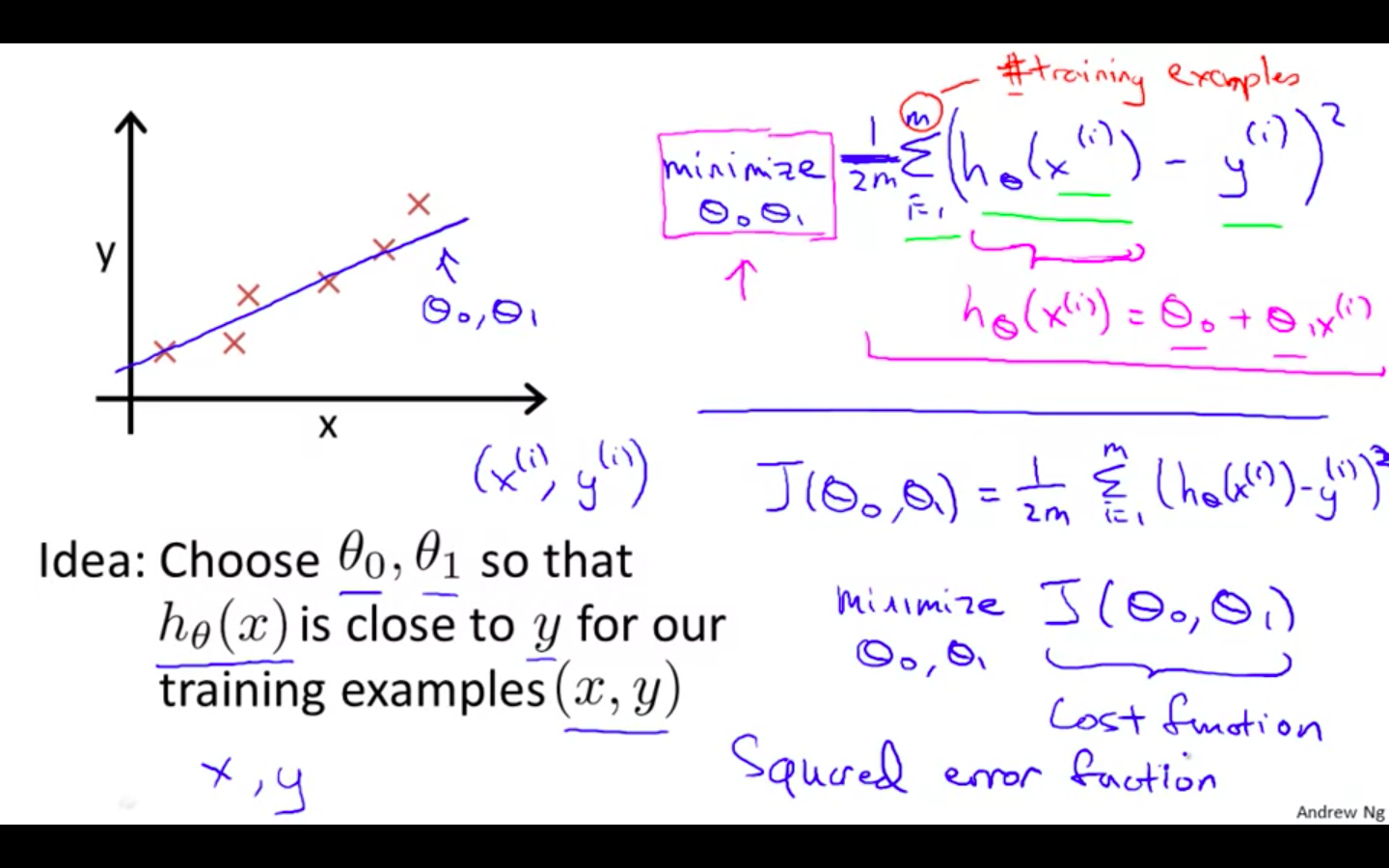
• Theta0 and theta1 are called the parameters.

• How to chose the parameters ?

  • Idea: Choose parameters so that the function of x is close to y for our training examples.

• Squared Error Function

  Mean Squared Error

  • Reasonable for most of the regression problems

Intuition 1

• The best possible line will be such so that the average squared vertical distances of the scattered points from the line will be the least.

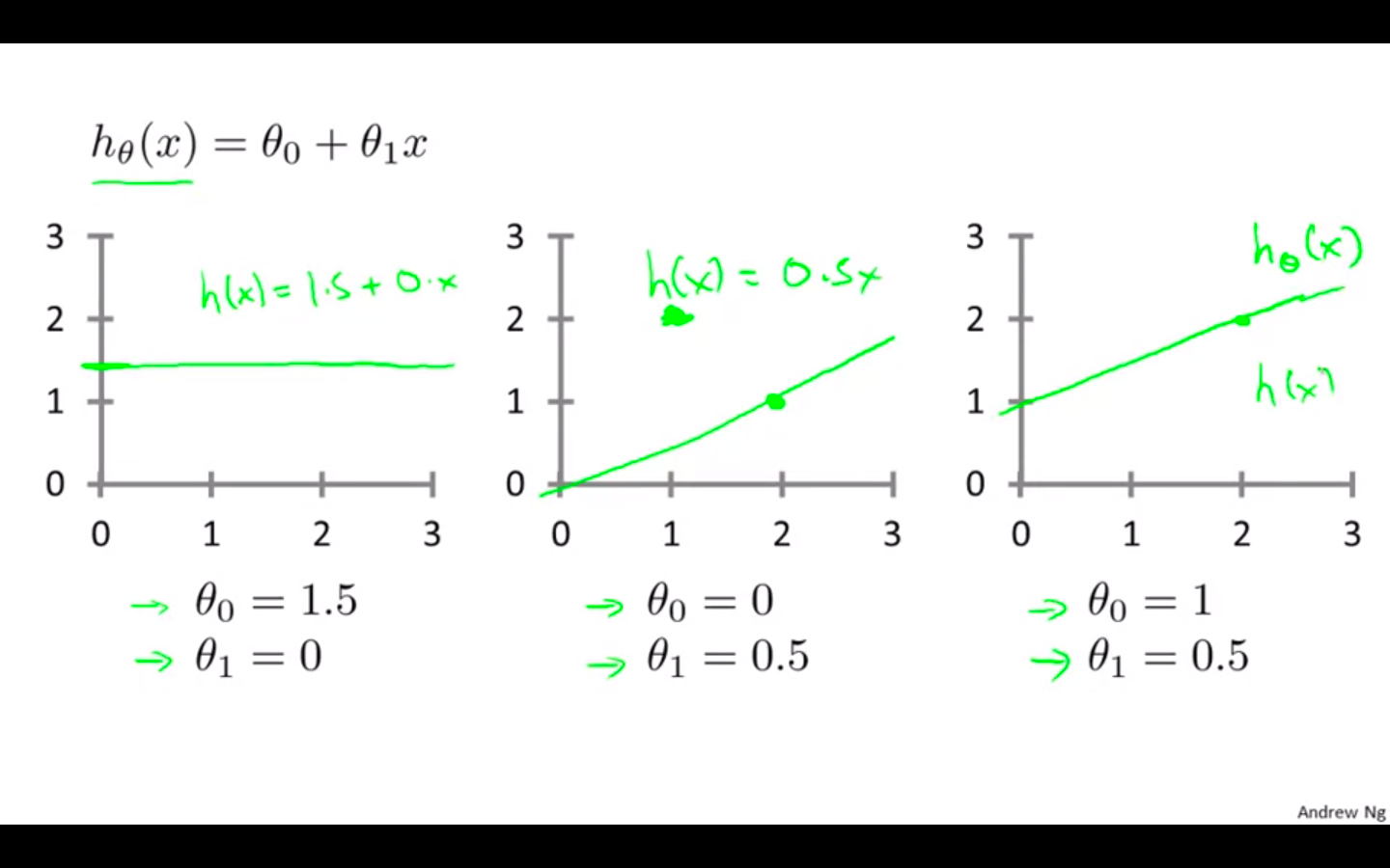
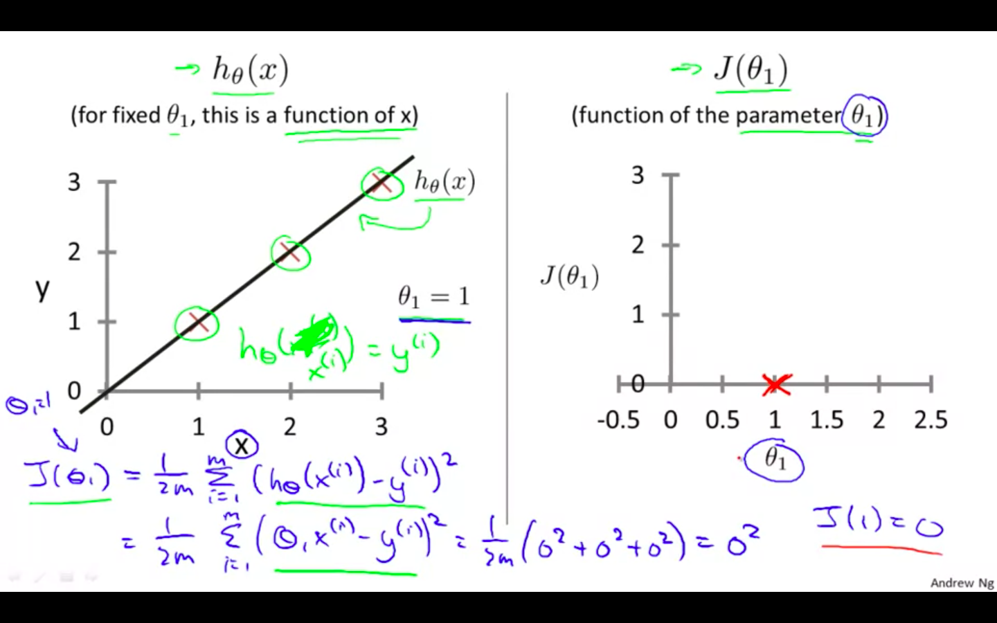
• Trying the function with the simplified version

  • Ideally, the line should pass through all the points of our training data set. In such a case, the value of J(theta0, theta1) will be 0.

  • Taking theta0 = 0 and changing the values of theta 1 to minimise the cost function.

  

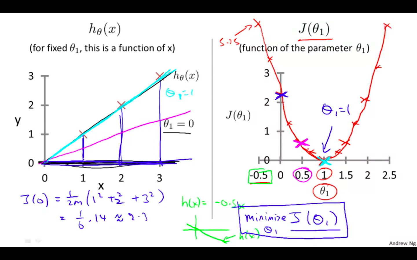
• First value : theta1 = 1

  

• Second value : theta1 = 0.5

  

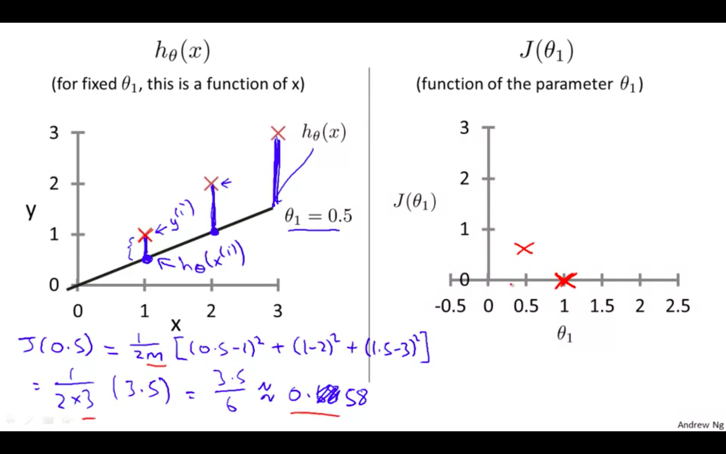
• Third value : theta1 = 0

  

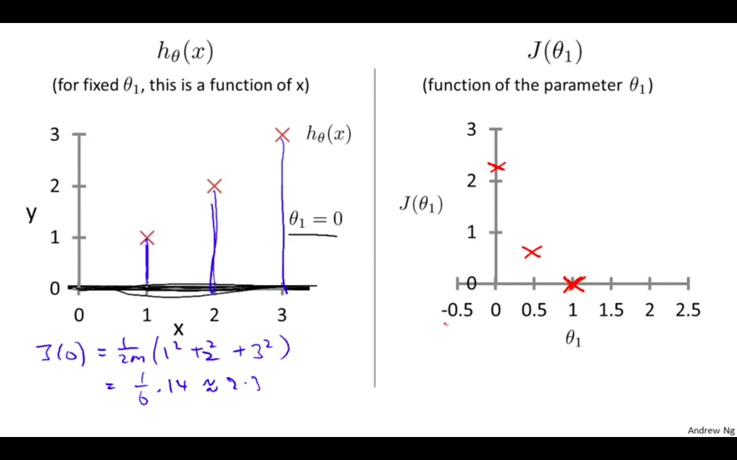
• We can plot different value using the function and then select the one which is of the least i.e minimise theta 1

  

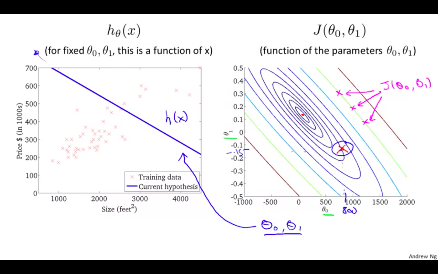
Intuition 2

• When calculating the cost function with two parameters the plot is in 3d graph.

  

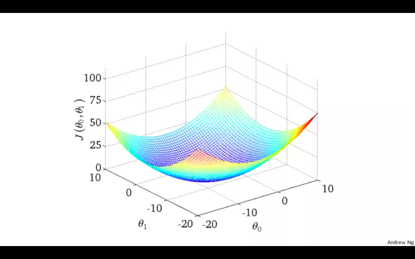
• It is also called as the convex function.

• Contour plane or figures are used in the diagrams.

• A contour plot is a graph that contains many contour lines.

• A contour line of a two variable function has a constant value at all points of the same line.

• Hypothesis 1

  

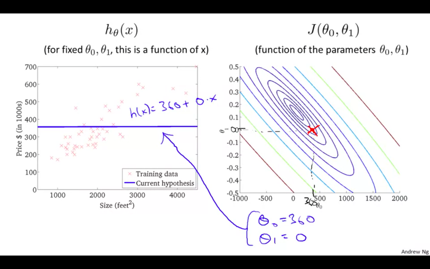
• Hypothesis 2

  

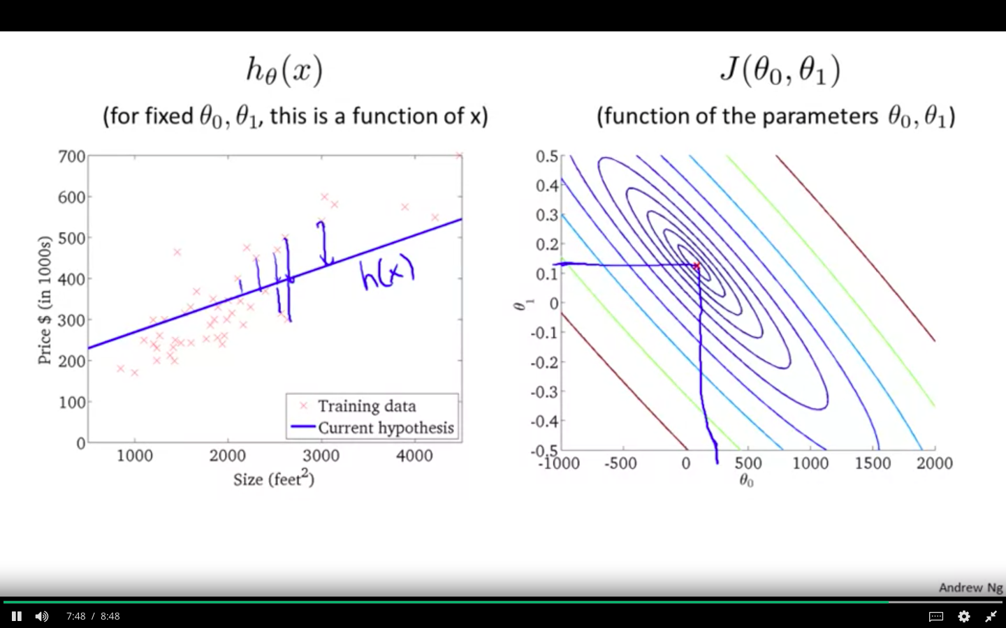
• Hypothesis 3

  

Parameter Learning

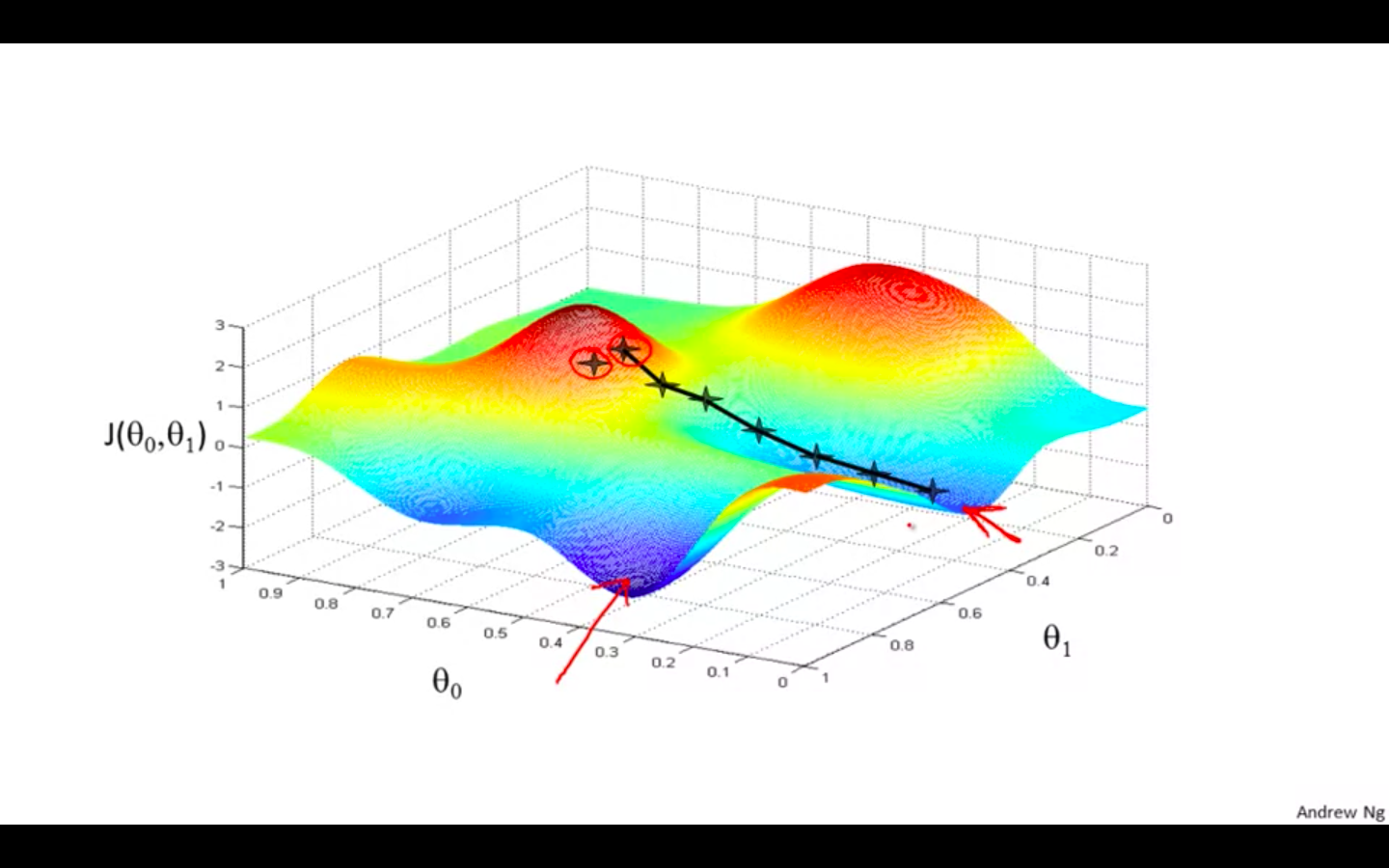
Gradient Descent

• We have some cost function

  • we want the minimum of that function

  

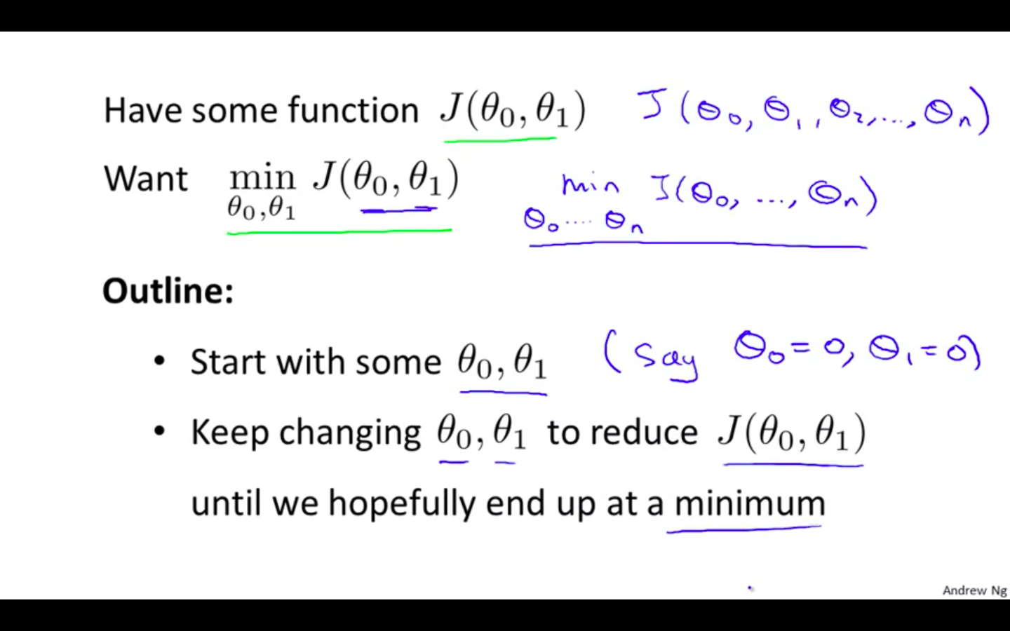
• Example

  • If this is a terrain and we are standing on a hill (random point selected to initialise).

  • Our aim is to come to lowest point on the terrain.

  • So we make decision of taking step in which direction so we can reach the bottom.

  • But if we change the initial point, we can reach at different points or also called as local minimum.

  

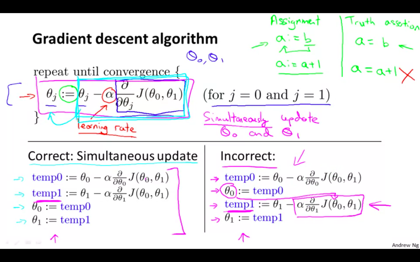
• Formula

  • := is called as the assignment operator

  • alpha is the learning rate

    • It determines the size of the step taken to reach bottom.

    • Bigger the alpha, bigger the step and vice versa.

  • Simultaneous update is required

  

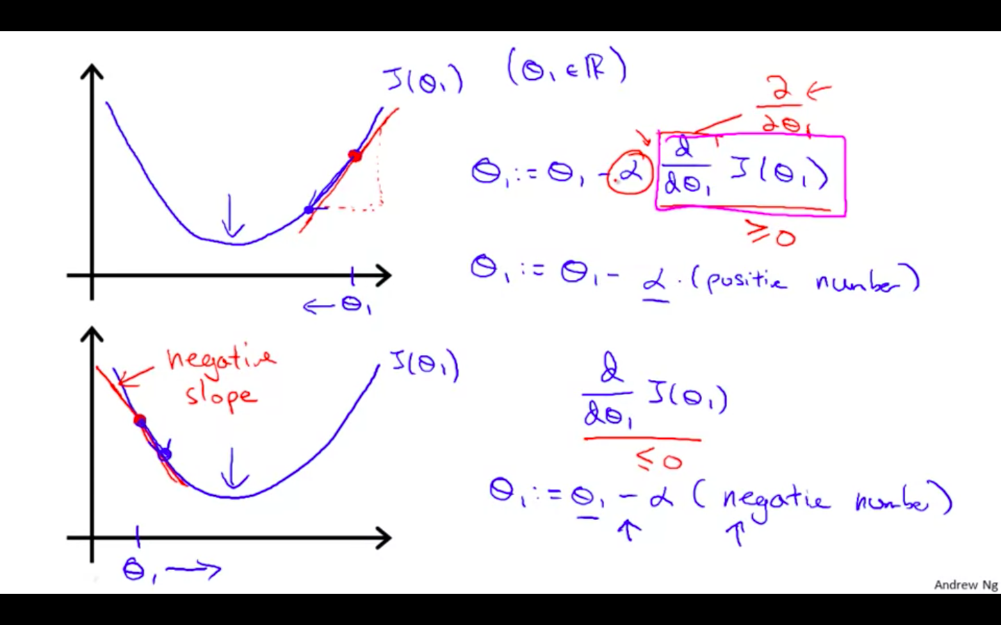
Intuition

• Gradient Descent with 1 parameter

  • The following graph shows that when the slope is negative, the value of theta1​ increases and when it is positive, the value of theta1​ decreases.

  

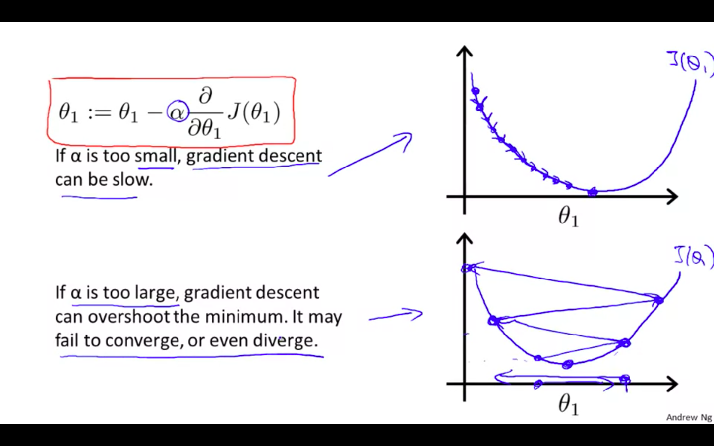
• Behavior change due to size of learning rate ( alpha )

  • If the size of the alpha is small

    • the process will be slow

  • If the size of the alpha is too large

    • it can overshoot the minimum

    • it may fail to or converge even diverge

  

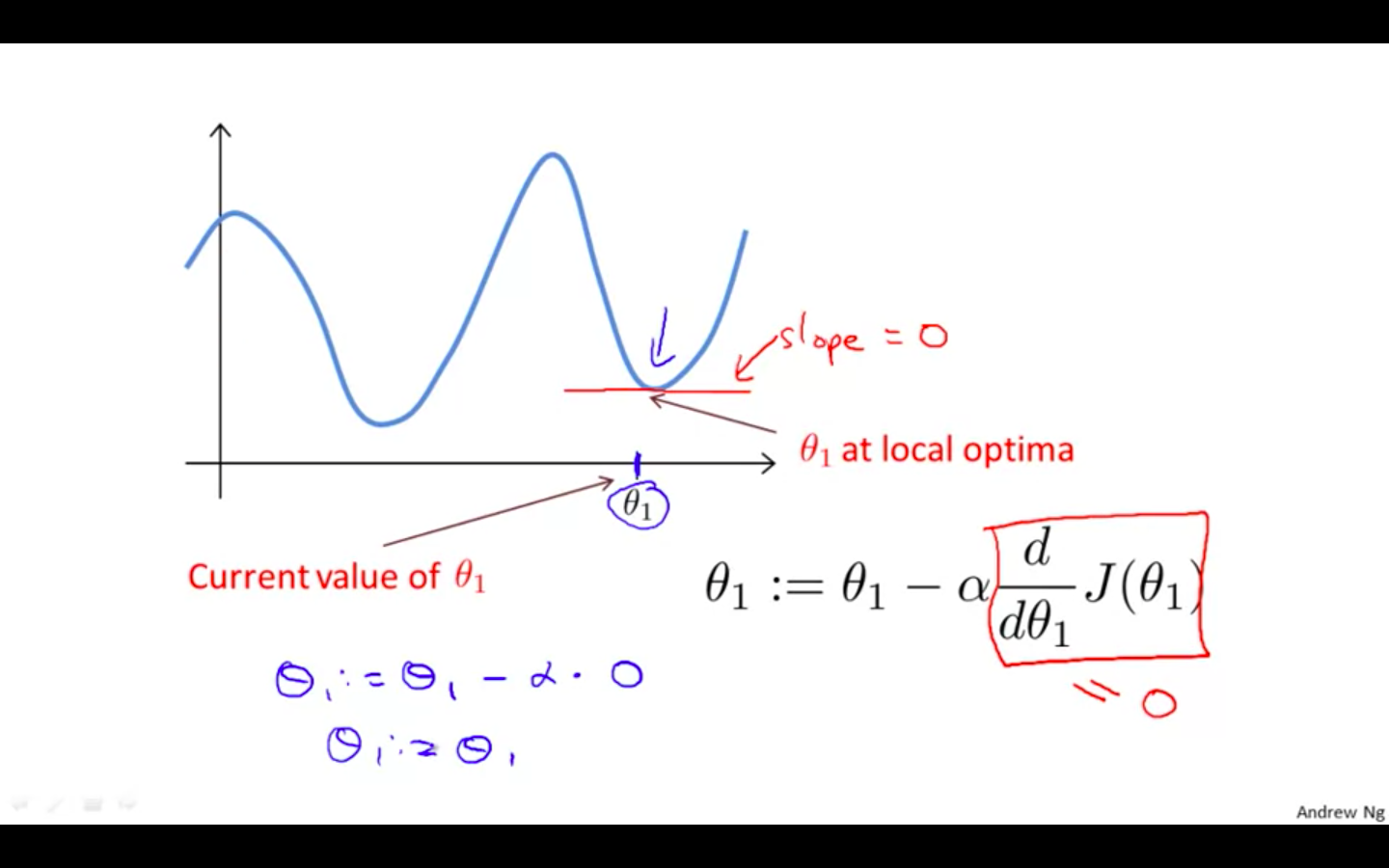
• What will happen if it reaches the local minimum ?

  • When it reaches the local minimum, the slope at that point would 0.

  • So the derivate will be zero and there will no change

  

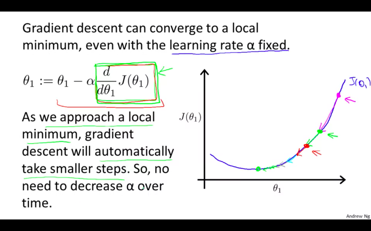
• What if the value of alpha is fixed ?

  • It will converge to a local minimum

  • It will automatically take smaller steps

  • No need to decrease alpha over time

  

  Gradient Descent For Linear Regression

  • Concept

    • Two Formula

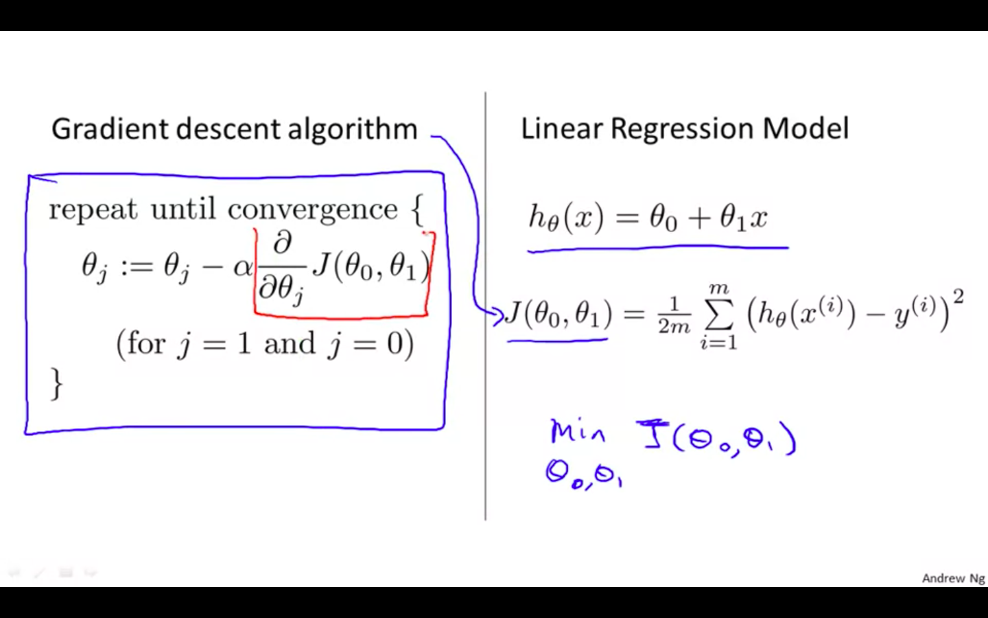
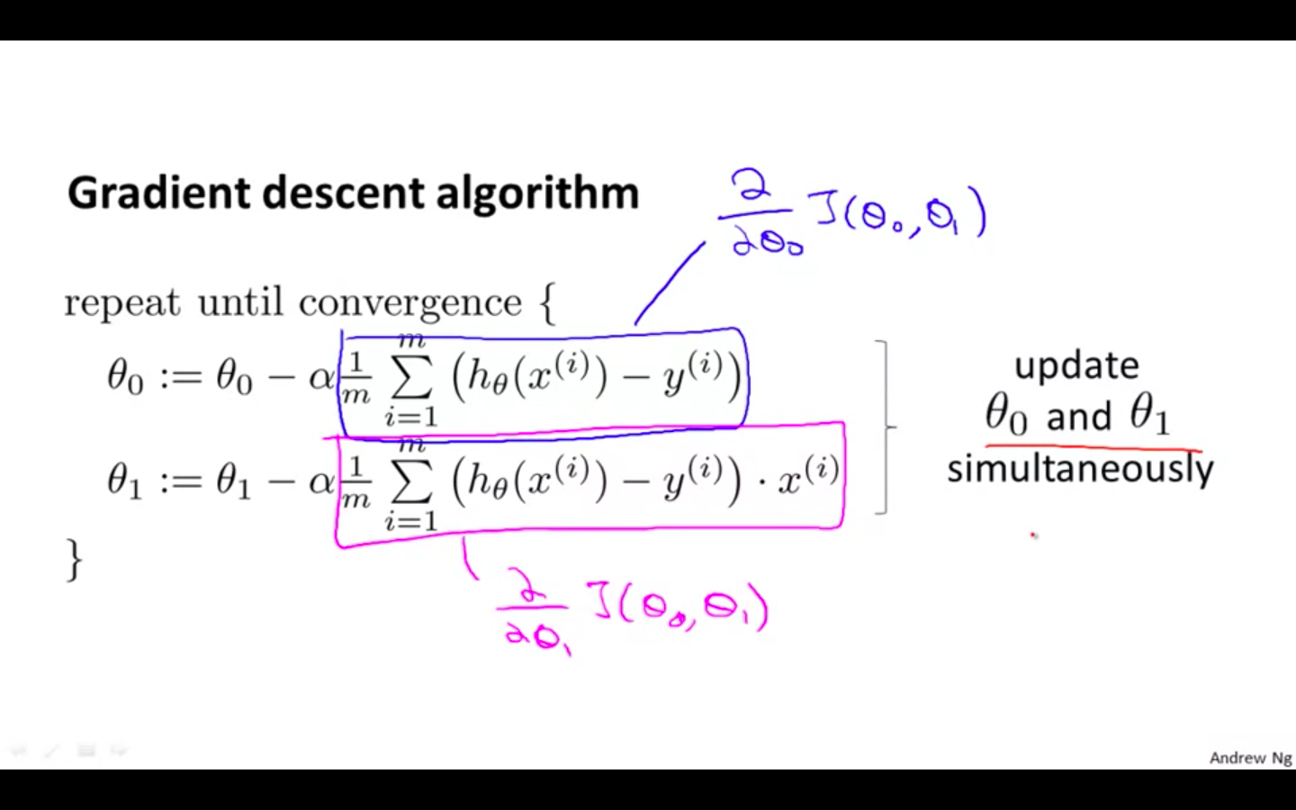
      • Gradient Descent Algorithm

      • Linear Regression Model

    • Minimise the cost function of linear regression using gradient descent

    

• Proof

  • Deriving the values of the parameters (theta0 and theta1)

  

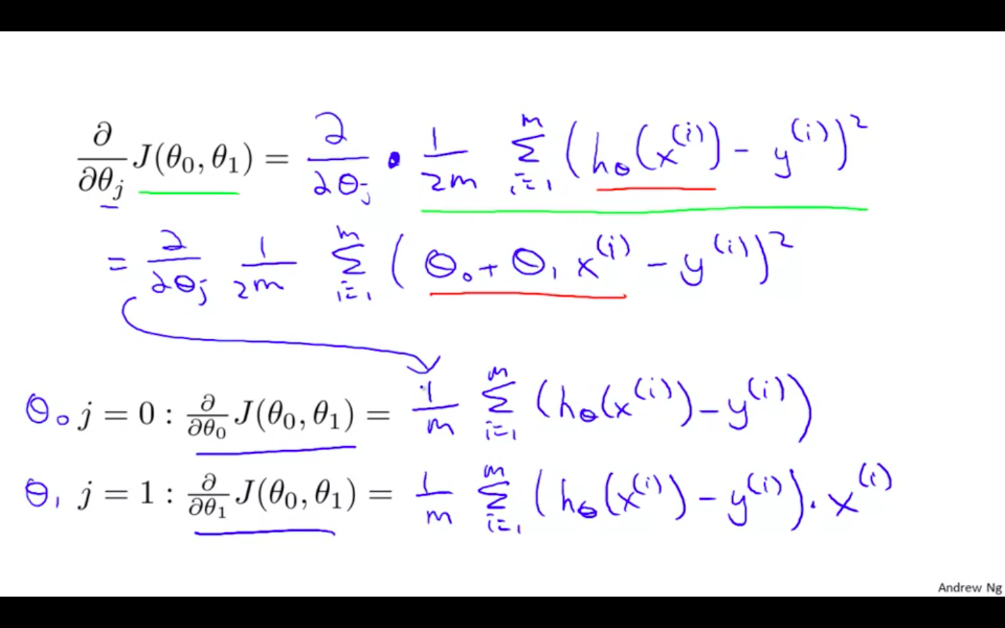
• Modified Algorithm

  • Algorithm after solving

    • updating parameters simultaneously is needed

  

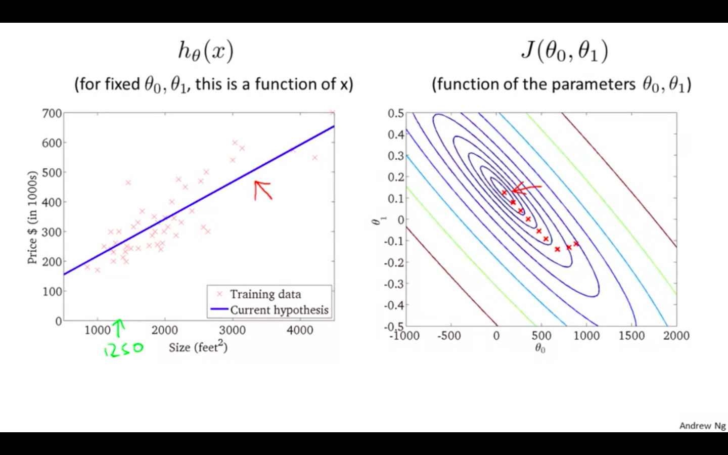
• Results Of Gradient Descent

  • Linear regression has no local minimum, only one global minimum.

  

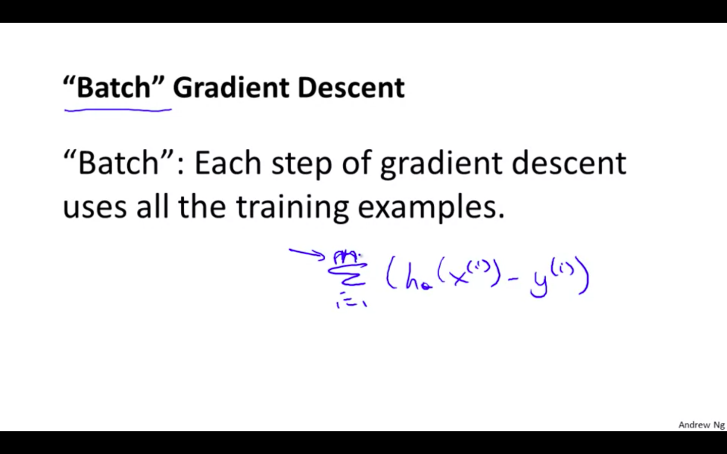
• Batch Gradient Descent

  • This type of gradient descent is called as “Batch” Gradient Descent.

  • The name “Batch” is given because it uses all the training examples.

  

Linear Algebra

Matrices and Vectors

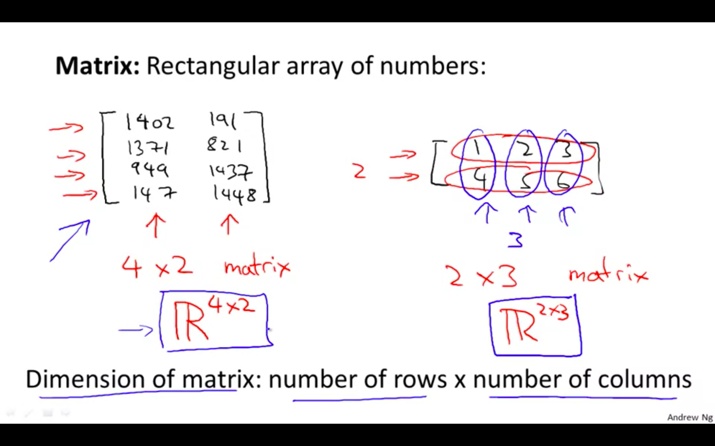
• Matrices

  • It is a multi-dimensional array

  • Dimension of matrix = number of rows x number of columns

  

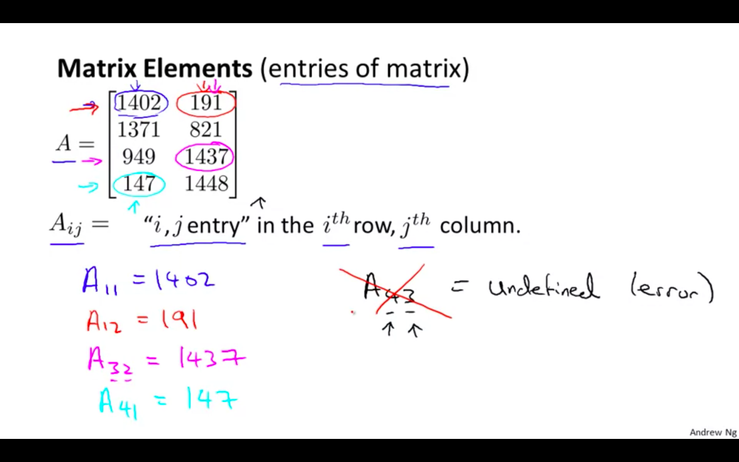
• Elements Of Matrices

  • Elements of the matrix can be accessed using the i or j the term

  • i th term = row && j th term = column

  

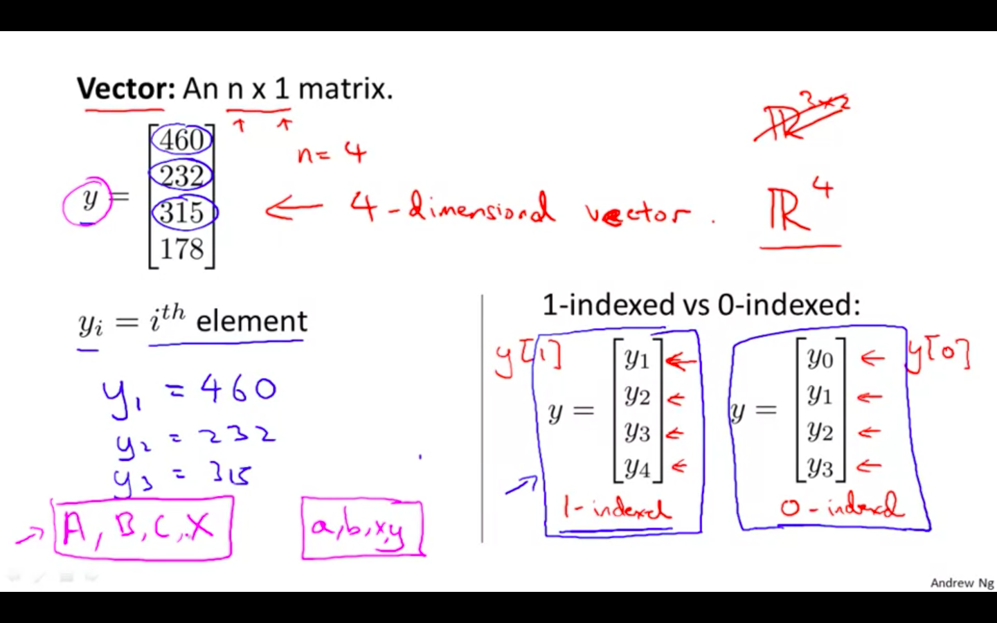
• Vectors

  • It a a matrix with on column and ‘n’ rows.

  

• In general, all our vectors and matrices will be 1-indexed. Note that for some programming languages, the arrays are 0-indexed.

• Matrices are usually denoted by uppercase names while vectors are lowercase.

• “Scalar” means that an object is a single value, not a vector or matrix.

• Octave/Matlab Snippet

  • Code for matrices and vectors

% The ; denotes we are going back to a new row.
A = [1, 2, 3; 4, 5, 6; 7, 8, 9; 10, 11, 12]

% Initialize a vector
v = [1;2;3] hu

% Get the dimension of the matrix A where m = rows and n = columns
[m,n] = size(A)

% You could also store it this way
dim_A = size(A)

% Get the dimension of the vector v
dim_v = size(v)

% Now let's index into the 2nd row 3rd column of matrix A
A_23 = A(2,3)

Addition and Scalar Multiplication

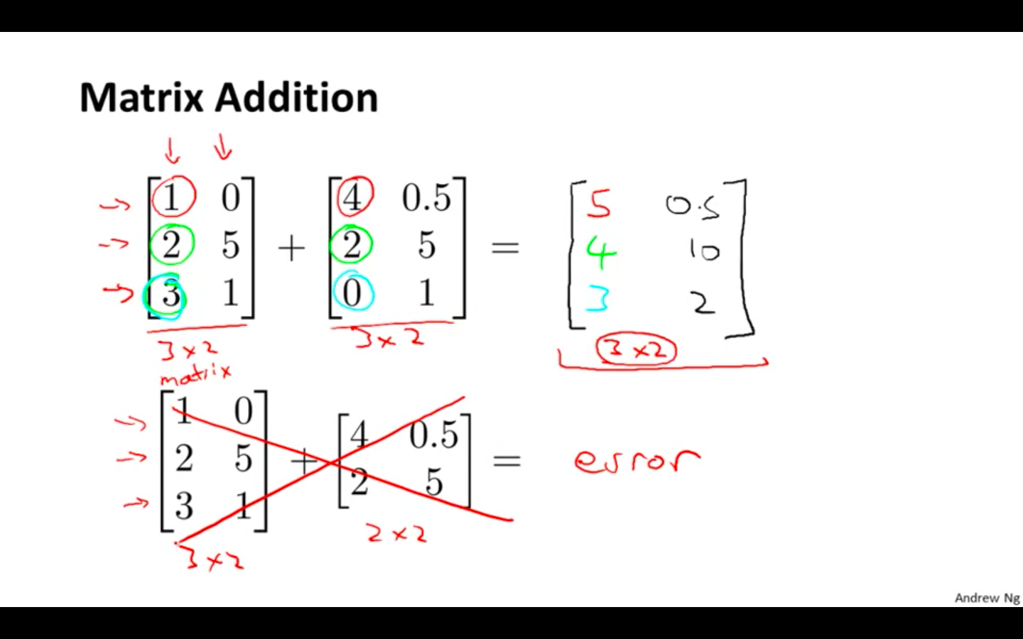
• Matrix Addition

  Subtraction

  • Only matrix with same dimensions can be operated.

  • Size of the output matrix would be same as the input matrix

  

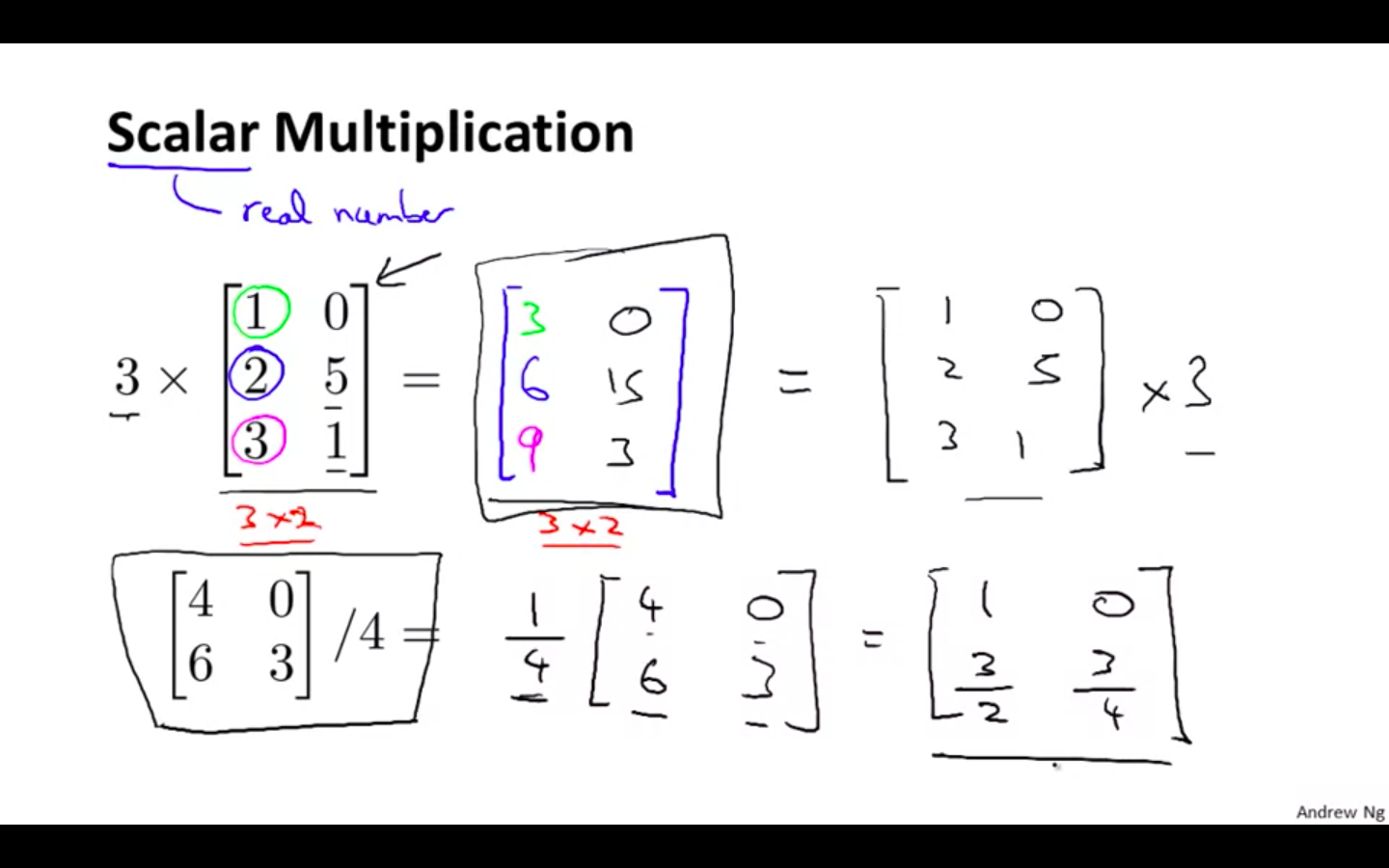
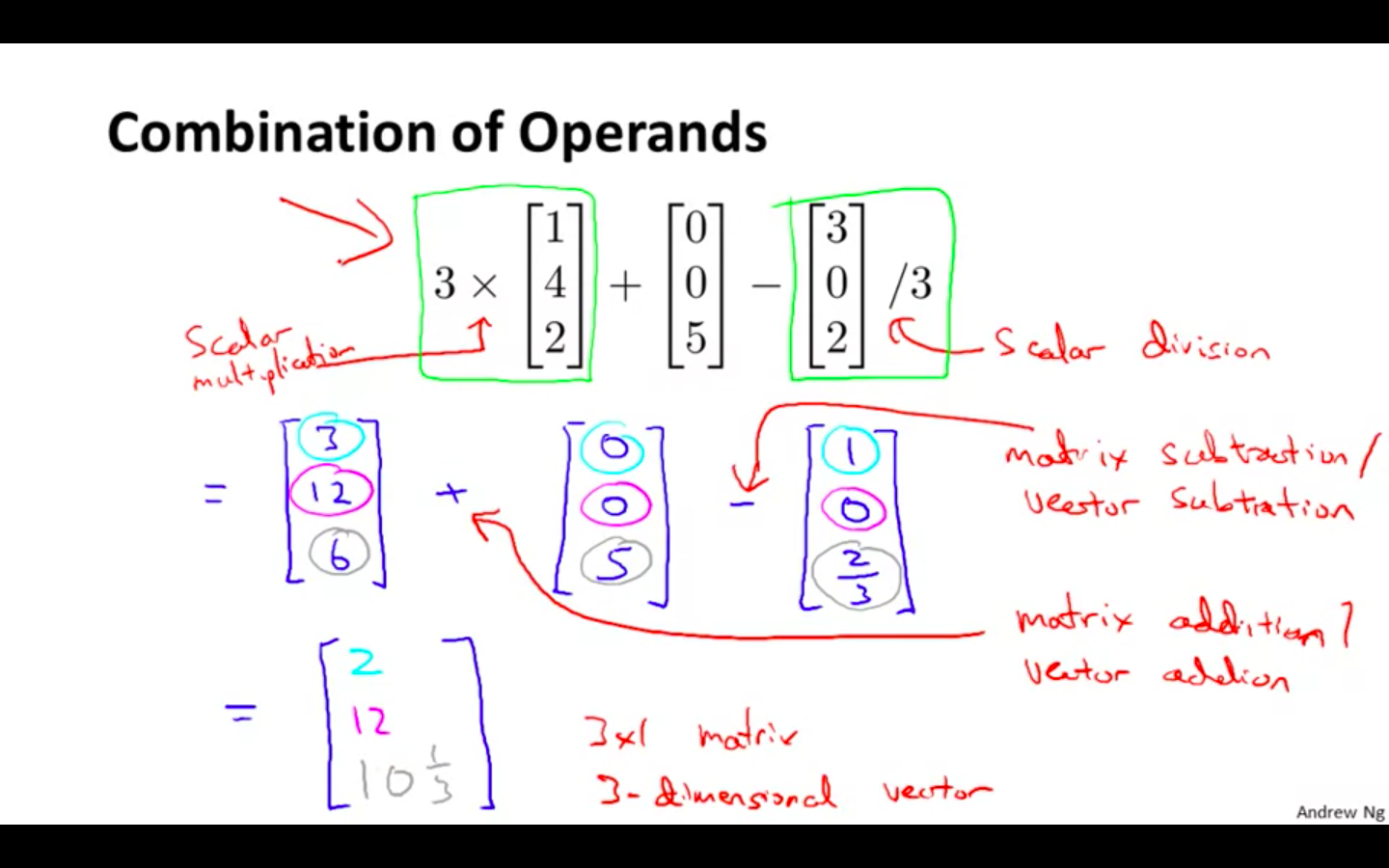
• Scalar Multiplication

  Division

  • Scalar gets multiplied or divided to each and every element of the matrix

  

• Combination of Operands

  • Many operations can be combined

  

• Octave/Matlab Snippet

  • Octave/Matlab commands for matrix addition and scalar multiplication.

% Initialize matrix A and B
A = [1, 2, 4; 5, 3, 2]
B = [1, 3, 4; 1, 1, 1]

% Initialize constant s
s = 2

% See how element-wise addition works
add_AB = A + B

% See how element-wise subtraction works
sub_AB = A - B

% See how scalar multiplication works
mult_As = A * s

% Divide A by s
div_As = A / s

% What happens if we have a Matrix + scalar?
add_As = A + s

Matrix Vector Multiplication

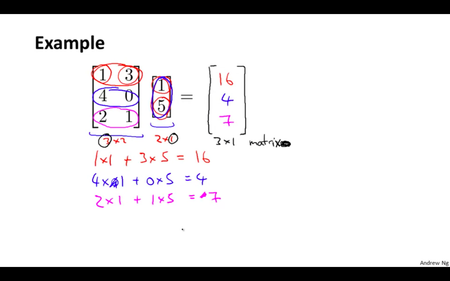
• Example 1

  • The result is a vector. The number of columns of the matrix must equal the number of rows of the vector.

  

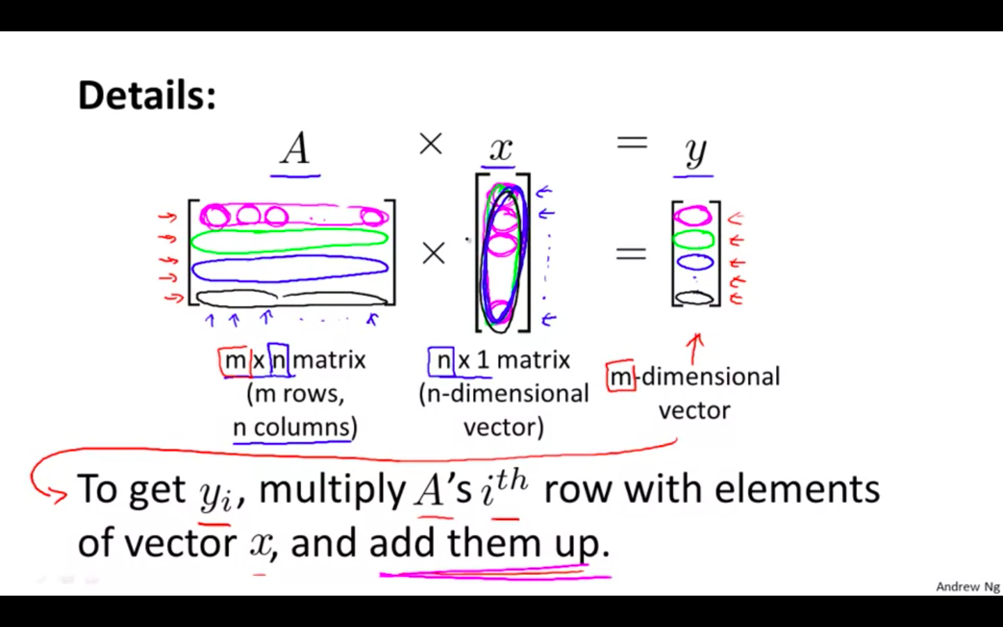
• Details

  • An m x n matrix multiplied by an n x 1 vector results in an m x 1 vector.

  

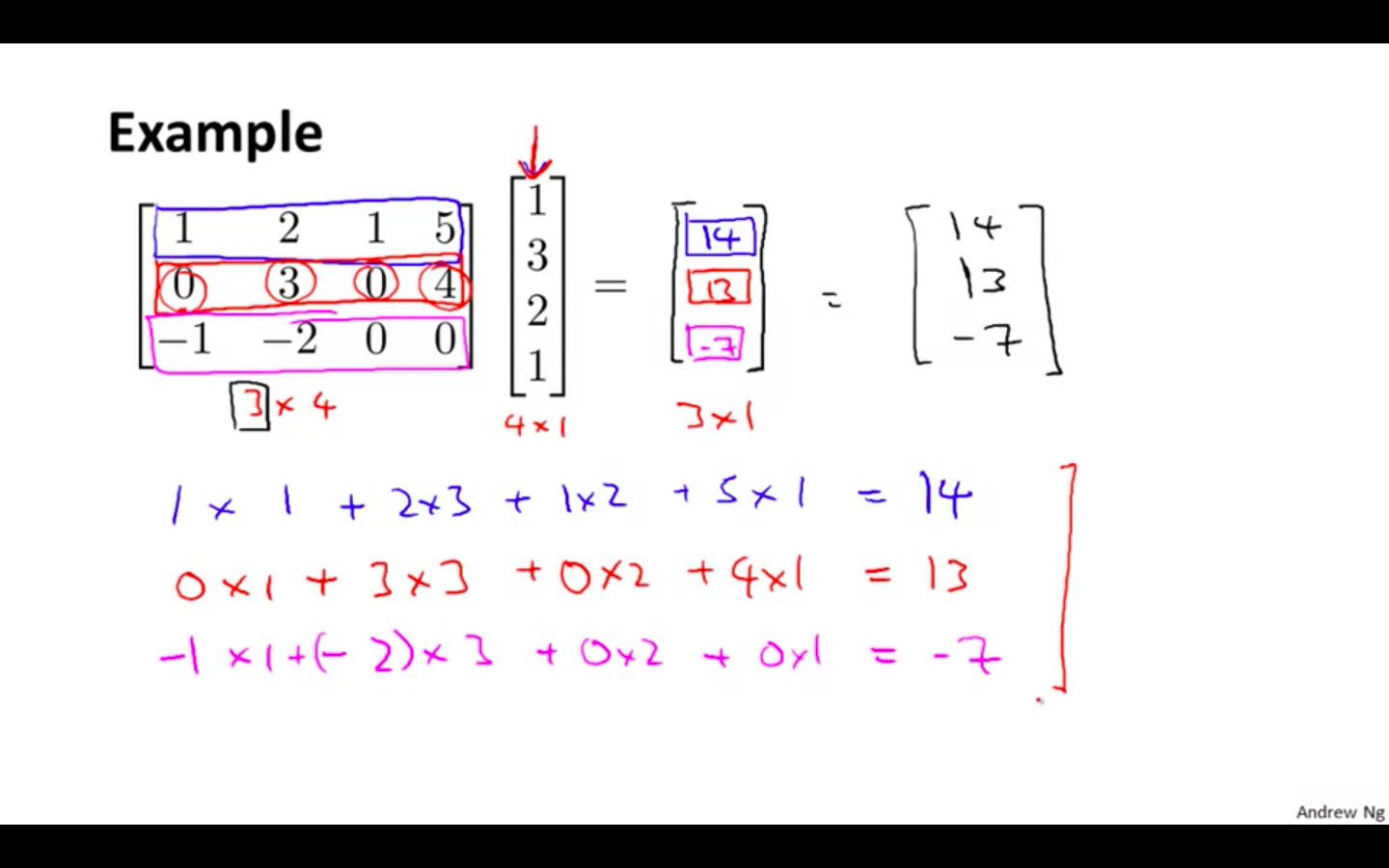
• Example 2

  

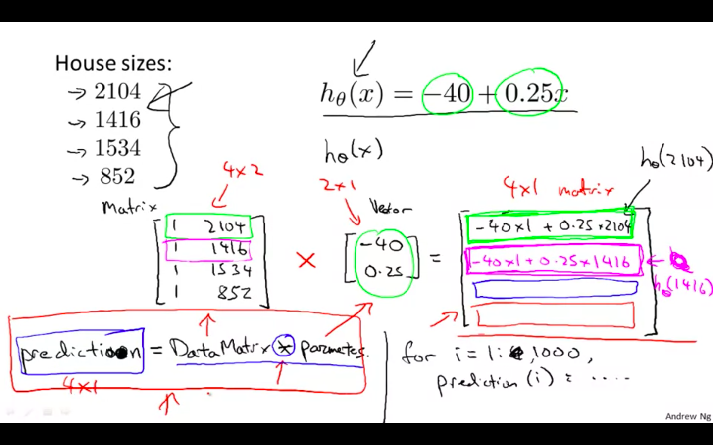
• Hypothesis Trick

  • Hypothesis can be applied to many values efficiently by using matrix-vector multiplication

  • Matrix would be the data set or the value on which hypothesis is to be applied

  • Vector would be the hypothesis

  • Output would be the predictions from the hypothesis

  

• Octave/Matlab Snippet

  • matrix-vector multiplication

% Initialize matrix A
A = [1, 2, 3; 4, 5, 6;7, 8, 9]

% Initialize vector v
v = [1; 1; 1]

% Multiply A * v
Av = A * v

Matrix Matrix Multiplication

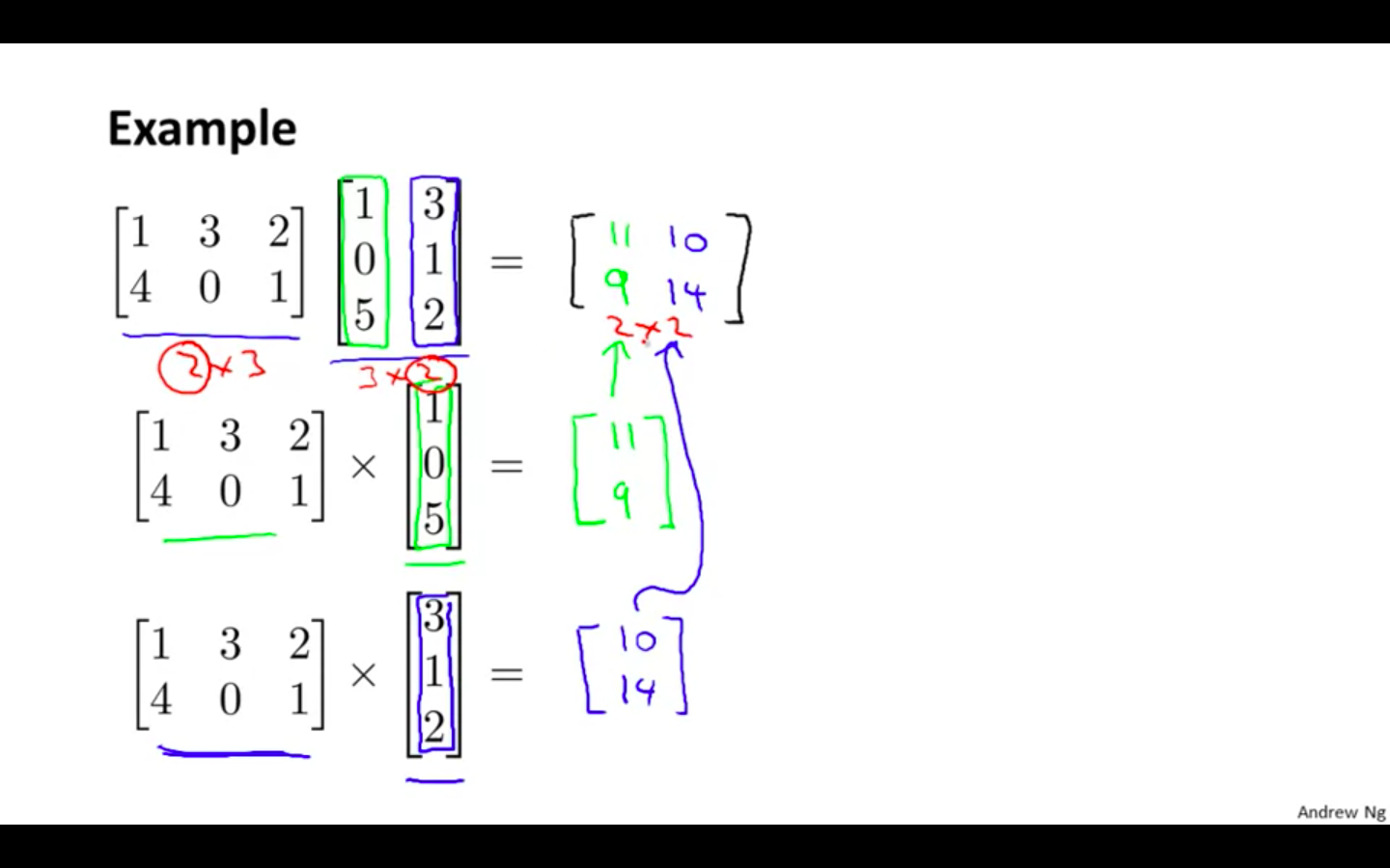
• Example 1

  • multiply two matrices by breaking it into several vector multiplications and concatenating the result.

  

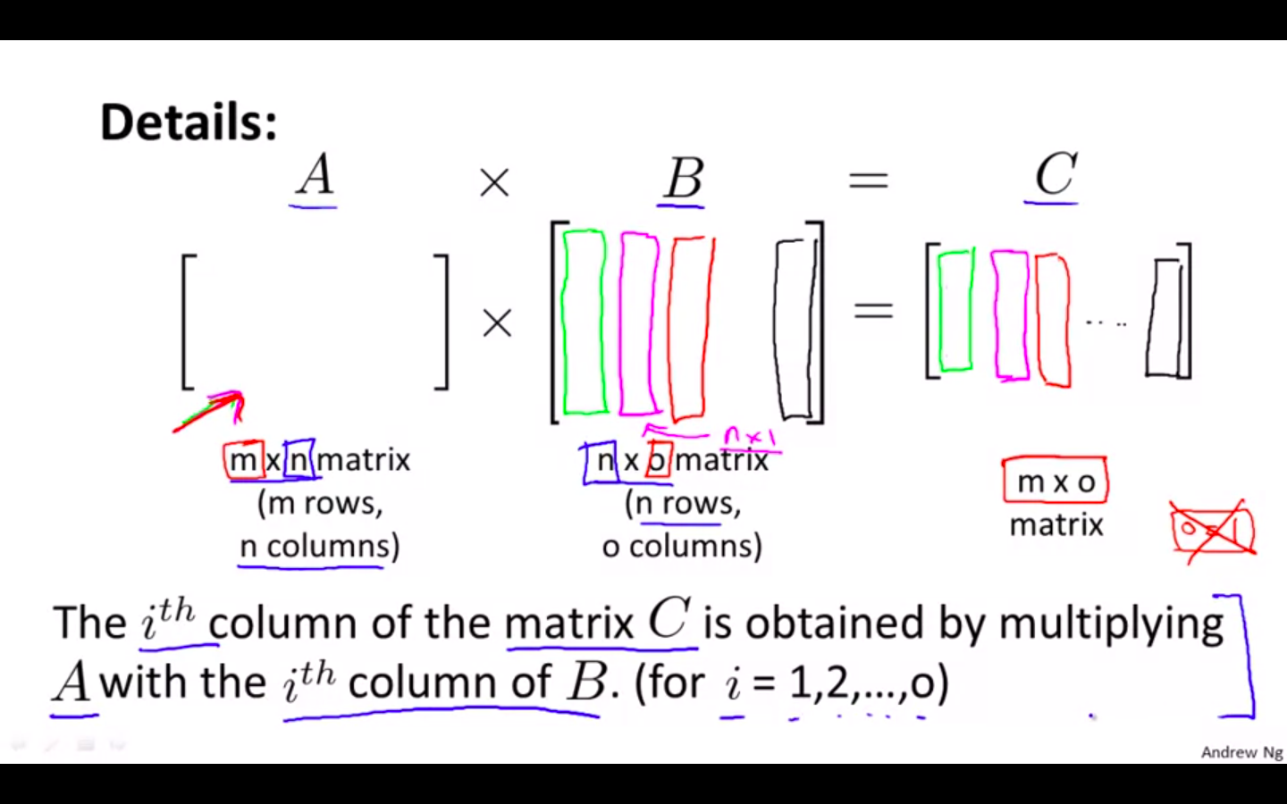
• Details

  • An m x n matrix multiplied by an n x o matrix results in an m x o matrix.

  • To multiply two matrices, the number of columns of the first matrix must equal the number of rows of the second matrix.

  

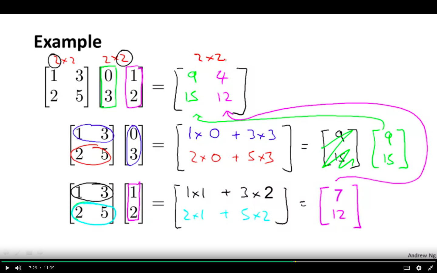
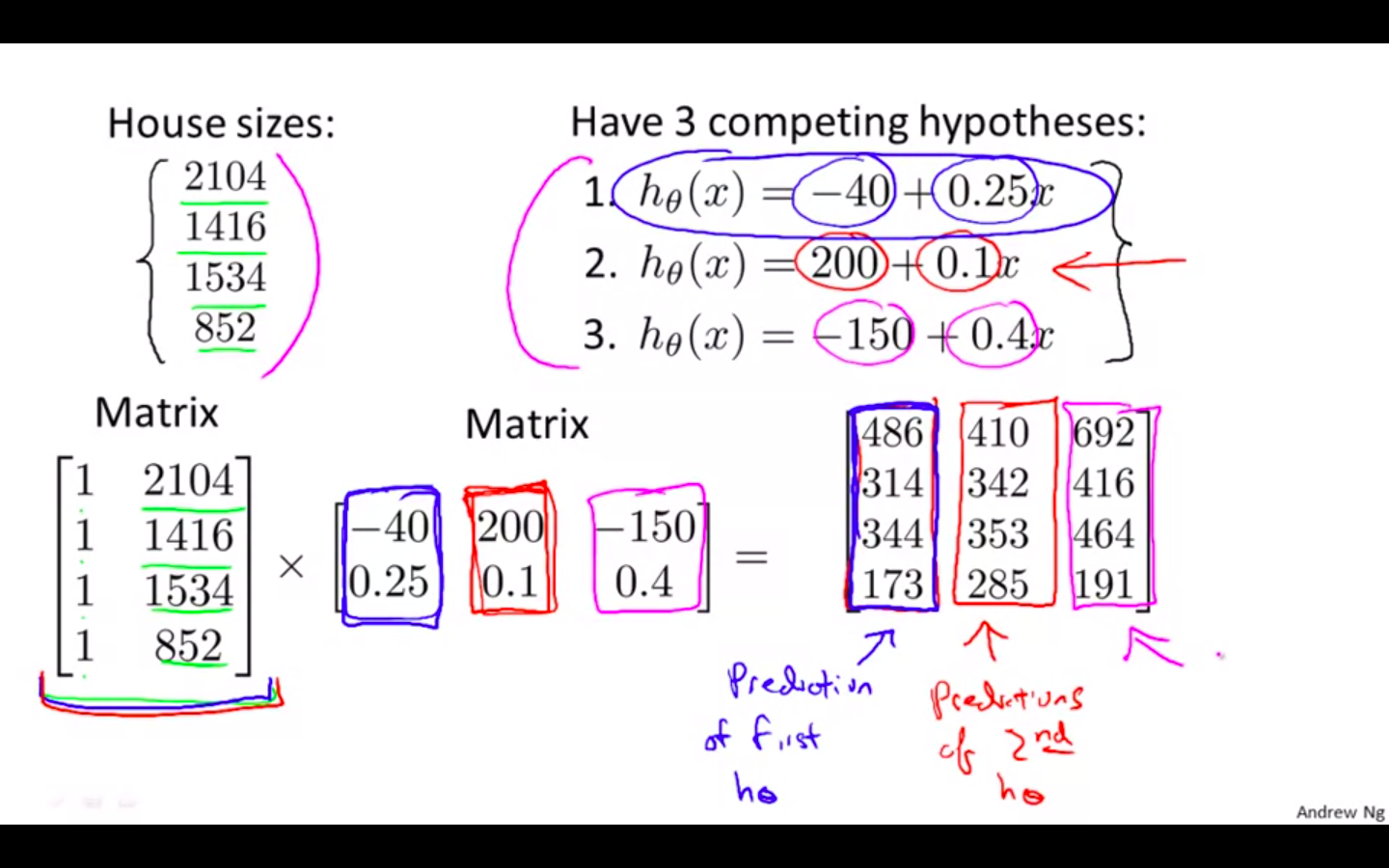
• Example 2

  

• Hypothesis Trick

  • Multiple hypothesis can be calculated using matrix matrix multiplication

  

• Octave/Matlab Snippets

  • matrix-matrix multiplication

% Initialize a 3 by 2 matrix
A = [1, 2; 3, 4;5, 6]

% Initialize a 2 by 1 matrix
B = [1; 2]

% We expect a resulting matrix of (3 by 2)*(2 by 1) = (3 by 1)
mult_AB = A*B

% Make sure you understand why we got that result

Matrix Multiplication Properties

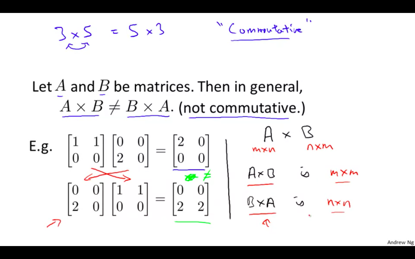
• Commutative

  • Matrices are not commutative

    • A _ B ≠ B _ A

  

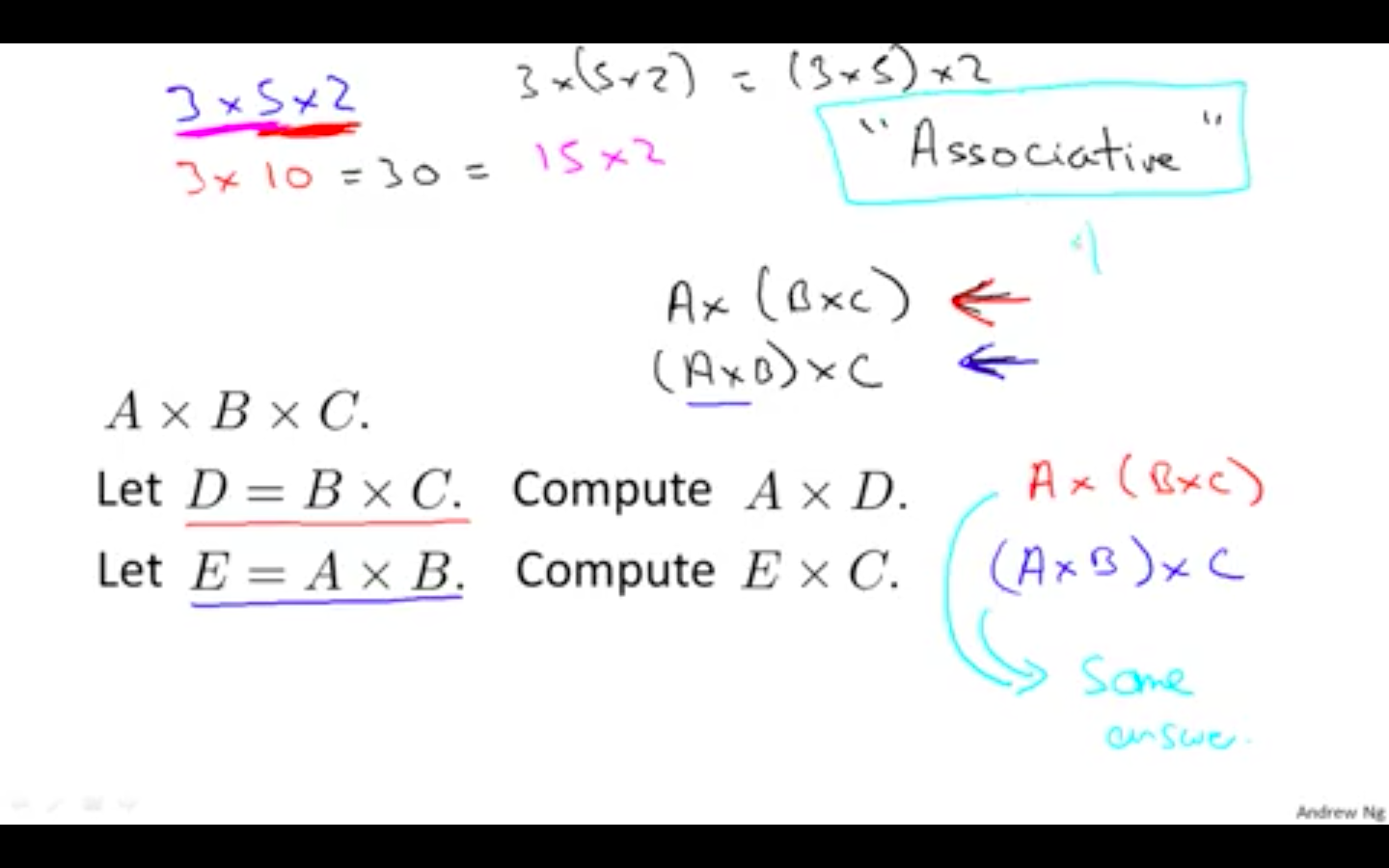
• Associative

  • Matrices are associative

    • (A _ B) _ C = A _ (B _ C)

  

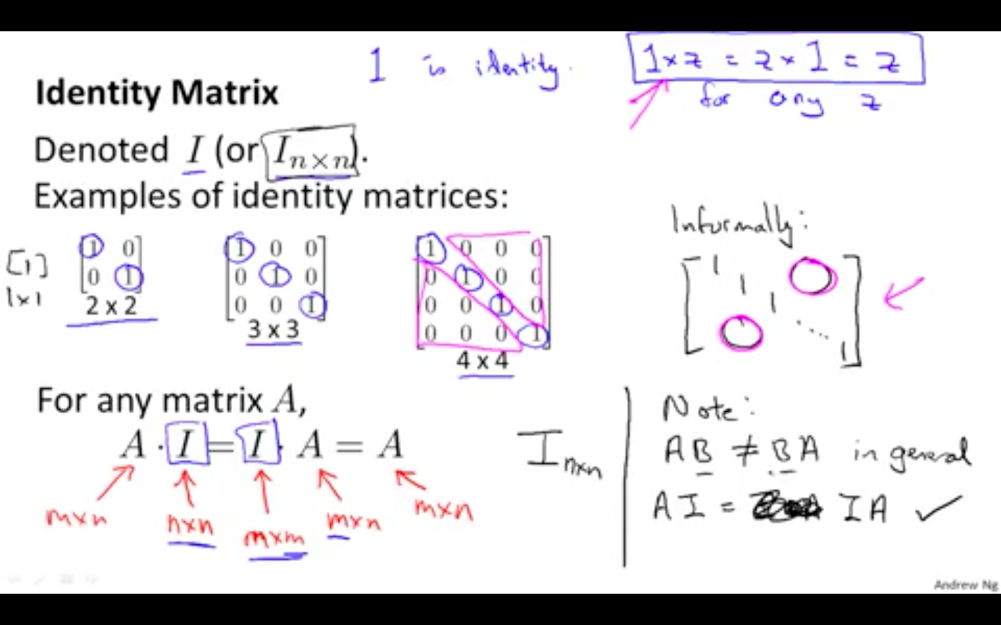
• Identity Matrix

  • The identity matrix, when multiplied by any matrix of the same dimensions, results in the original matrix.

  • When multiplying the identity matrix after some matrix (A∗I), the square identity matrix’s dimension should match the other matrix’s columns.

  • When multiplying the identity matrix before some other matrix (I∗A), the square identity matrix’s dimension should match the other matrix’s rows.

  

• Octave/Matlab Snippet

  -

% Initialize random matrices A and B
A = [1,2;4,5]
B = [1,1;0,2]

% Initialize a 2 by 2 identity matrix
I = eye(2)

% The above notation is the same as I = [1,0;0,1]

% What happens when we multiply I*A ?
IA = I*A

% How about A*I ?
AI = A*I

% Compute A*B
AB = A*B

% Is it equal to B*A?
BA = B*A

% Note that IA = AI but AB != BA

Inverse and Transpose

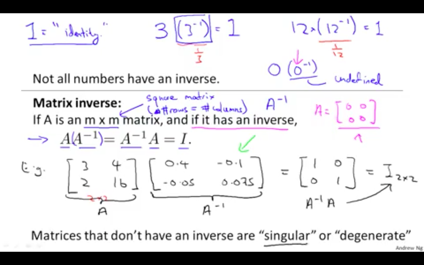
• Inverse

  • Multiplying by the inverse results in the identity matrix.

  • A non square matrix does not have an inverse matrix.

  • Matrices that don’t have an inverse are called singular or degenerate.

  

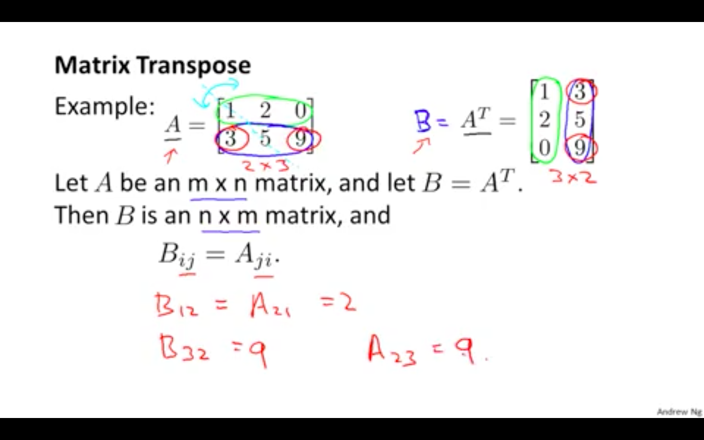
• Transpose

  • The transposition of a matrix is like rotating the matrix 90° in clockwise direction and then reversing it.

  

• Octave/Matlab Snippet

  • compute inverses of matrices in octave with the pinv(A) function and in Matlab with the inv(A) function.

  • We can compute transposition of matrices in matlab with the transpose(A) function

% Initialize matrix A
A = [1,2,0;0,5,6;7,0,9]

% Transpose A
A_trans = A'

% Take the inverse of A
A_inv = inv(A)

% What is A^(-1)*A?
A_invA = inv(A)*A

Lecture Presentation