Machine Learning By Andew Ng - Week 2

Multivariate Linear Regression

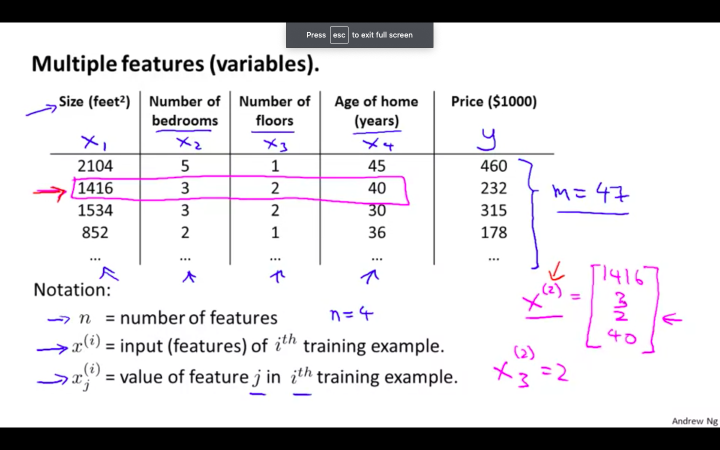
Multiple Features

• Linear regression with multiple variables is also known as “multivariate linear regression”.

• There can be ‘n’ number of features.

  • For the example of predicting the price of a house, features can be no. of bedrooms, no. of floors, age of home, size.

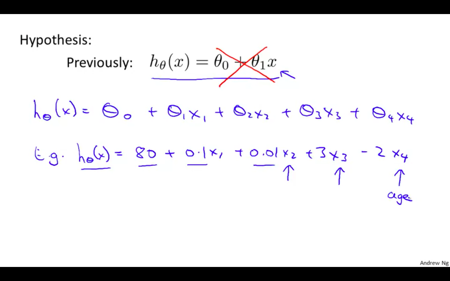
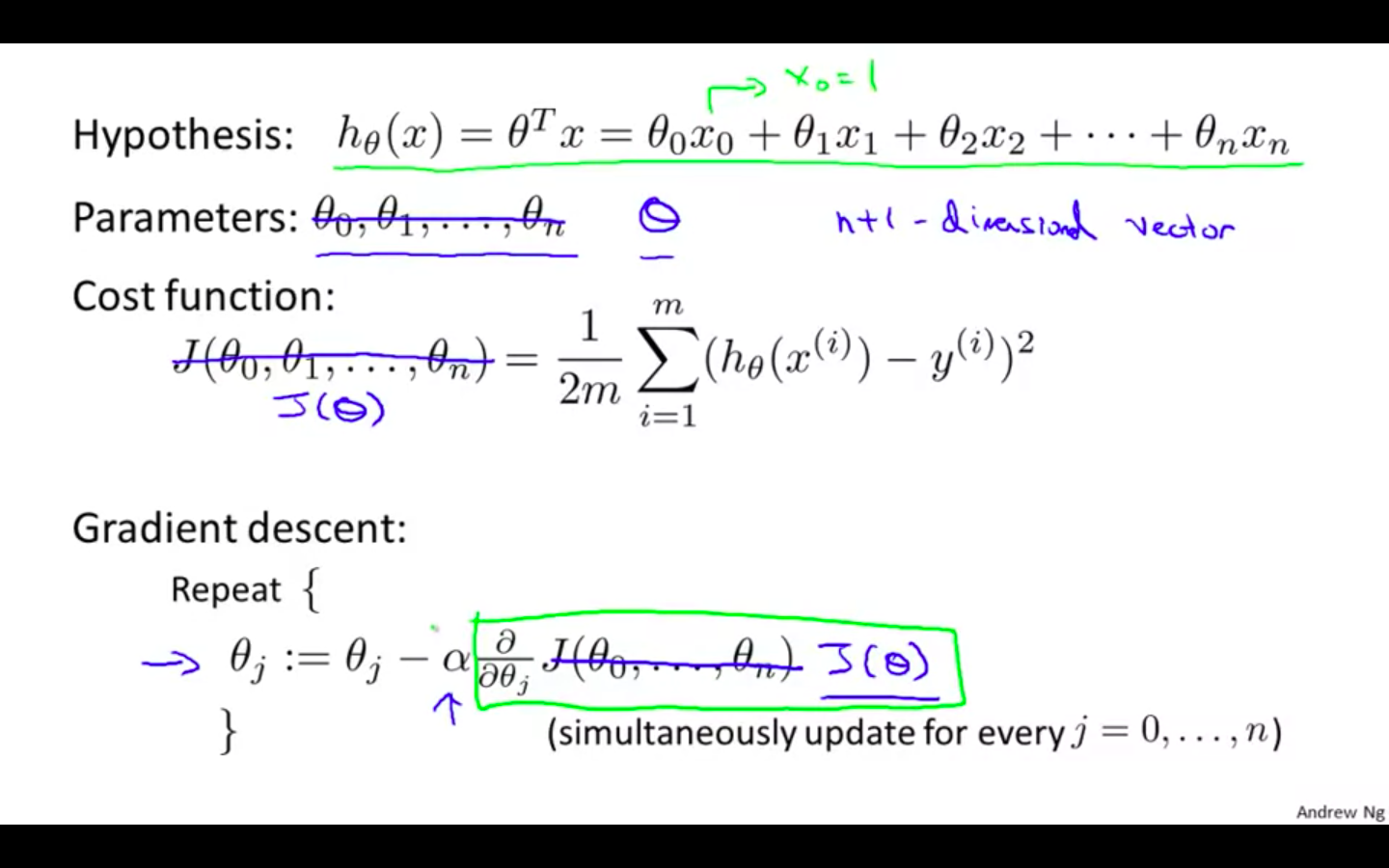
• Hypothesis

  • Number of parameters with their effect on the price of the house

  

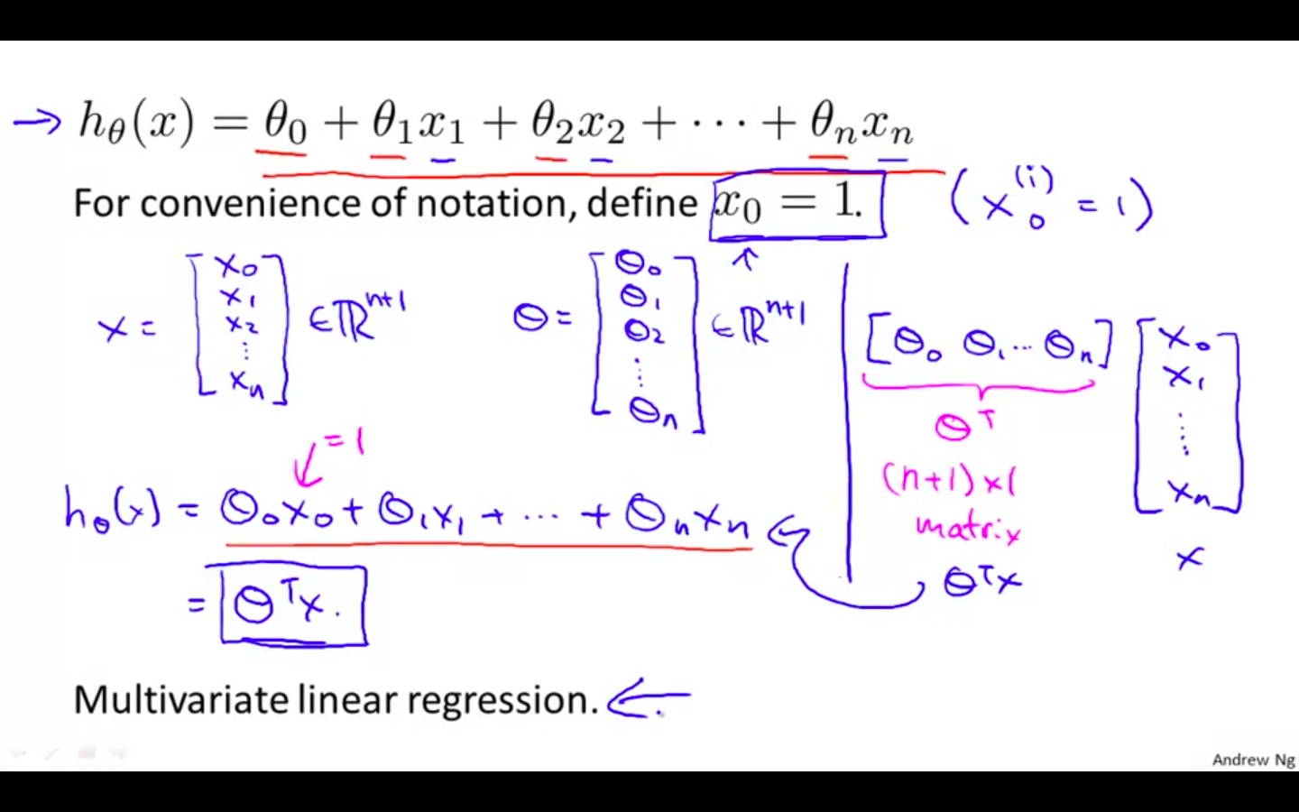
  • Taking x-zero as 1 for the convenience of notation

  • This is called as the Multivariate Linear Regression.

  

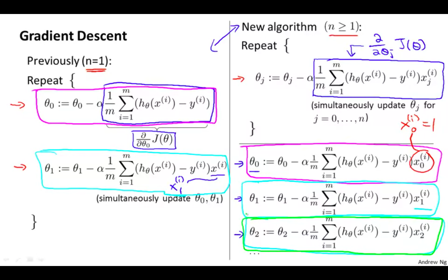
  Gradient Descent for Multiple Variables

  • Concept

    

  • Comparison between Gradient Descent with one variable and Gradient Descent with multiple variable

    

  Gradient Descent In Practice I - Feature Scaling

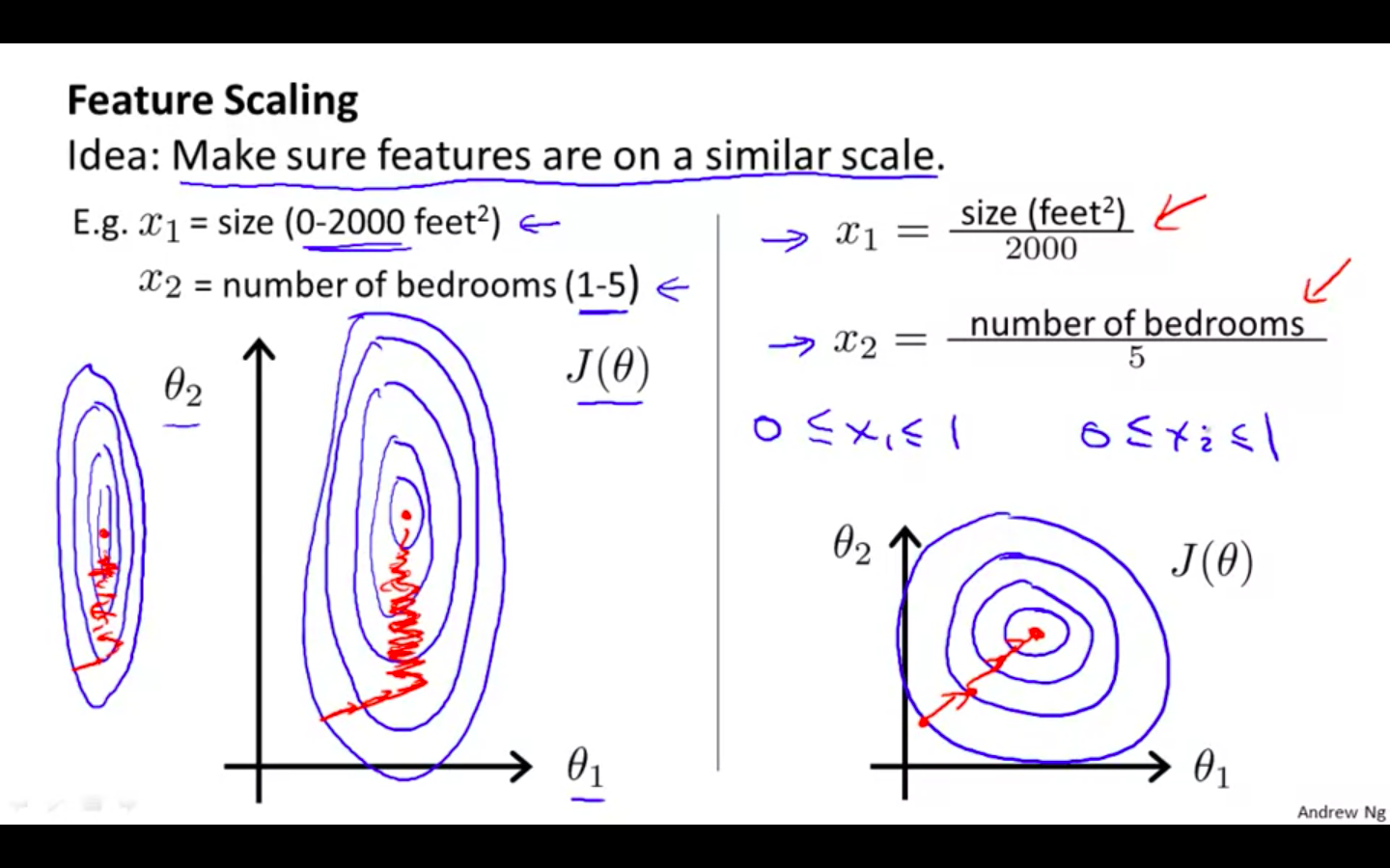
  • Features Scaling

    • Idea: Make sure features are on a similar scale

    • This is because θ will descend quickly on small ranges and slowly on large ranges, and so will oscillate inefficiently down to the optimum when the variables are very uneven.

    • If they are not on a similar scalar then the contours will be very elliptical

      • Gradient Descent will take more iteration to converge. i.e more time and power

    • If the features are on the similar scale, contours would be spaced and gradient descent would take less iteration to converge

    

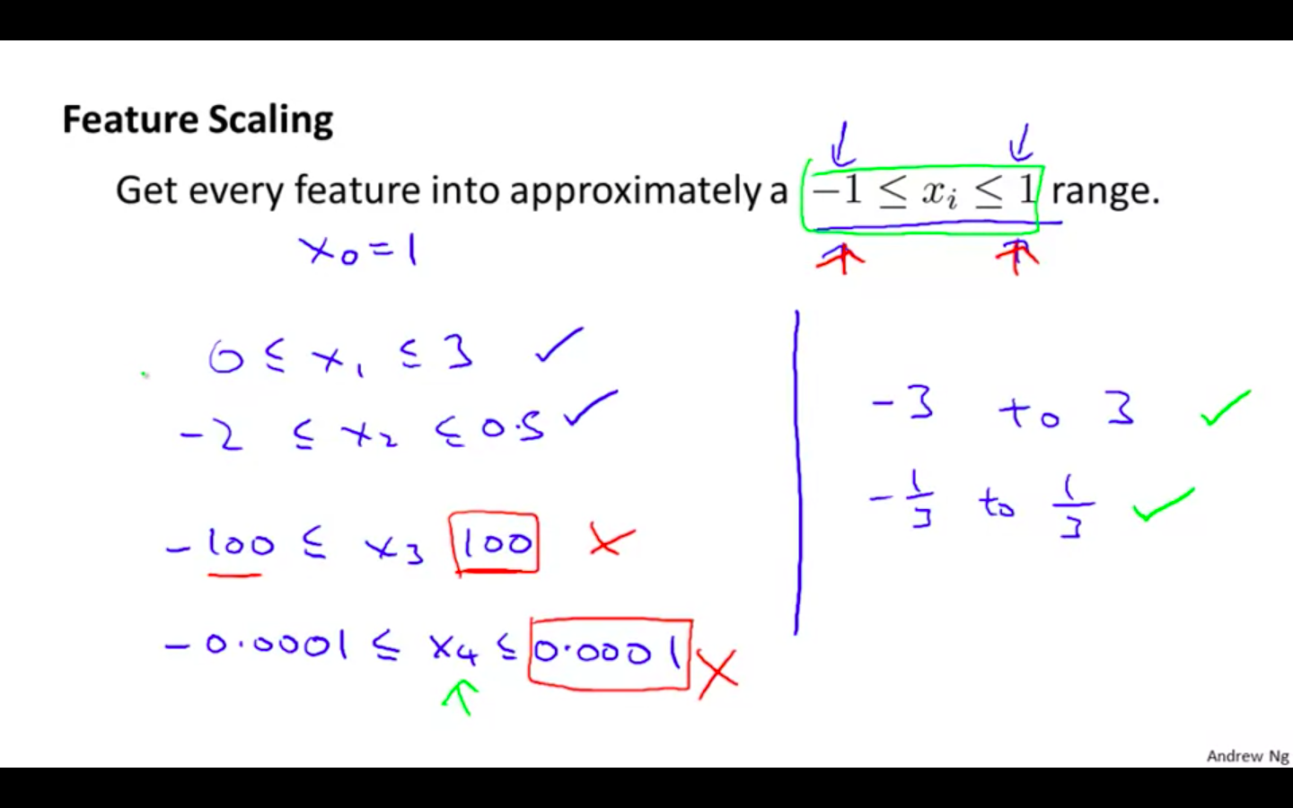
    • Feature should range between -1 ≤ x ≤ 1

      • +3, -3 = max

      • 1/3, -1/3 = min

    

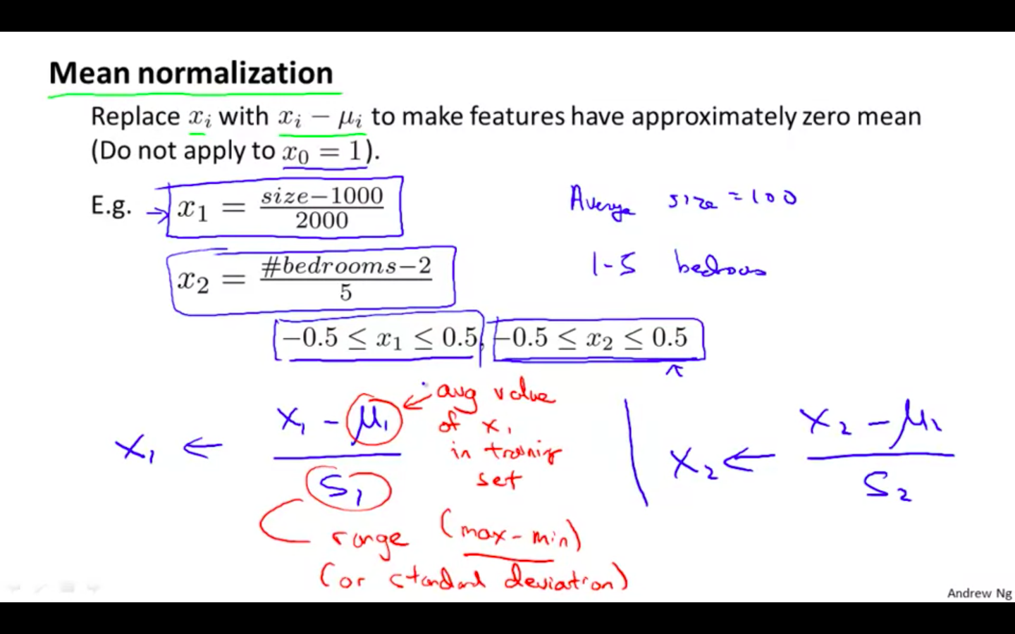
  • Mean Normalisation

    • Replace x with x - average value in the training set

    • Do not apply to x-zero = 1

    • This results in approximately zero mean.

    • x = x - average value on training set / s - range ( max - min )

      

Gradient Descent In Practice II - Learning Rate

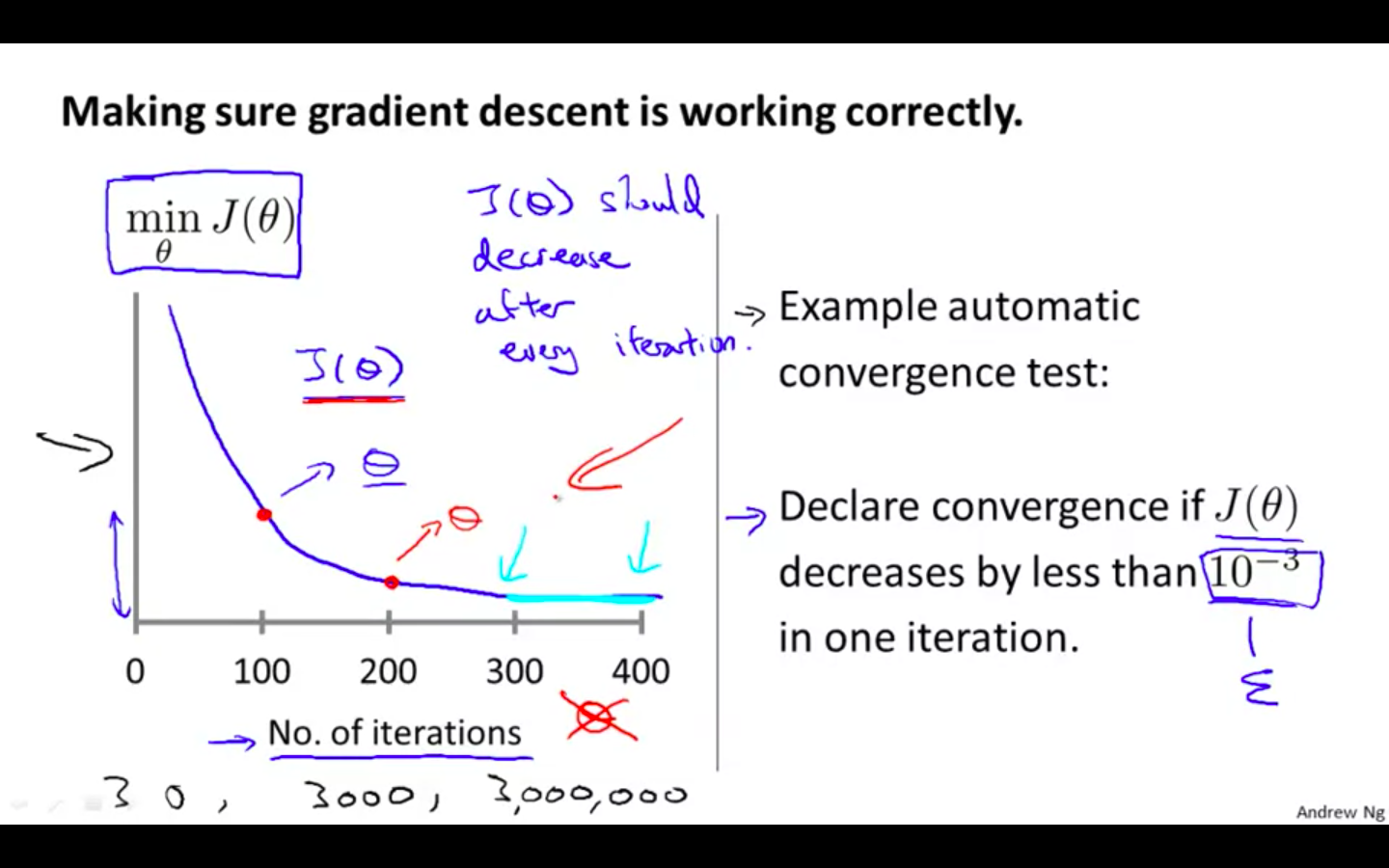
• “Debugging”: How to make sure gradient descent is working correctly

  • Plot the graph, on x-axis is the iteration and on y-axis value of cost function

    

  • Automatic convergence test can be implemented

    • Declare convergence if J(θ) decreases by less than E in one iteration, where E is some small value such as 10^-3

• How to choose learning rate alpha

  • It has been proven that if learning rate α is sufficiently small, then J(θ) will decrease on every iteration.

  

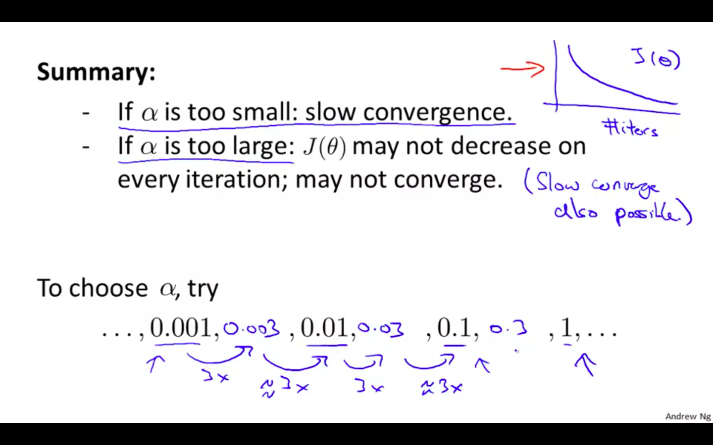
  • Summary

    • Try with some range of values

    • alpha is too small : slow convergence

    • alpha is too large : may not decrease on every iteration, may not even converge

    

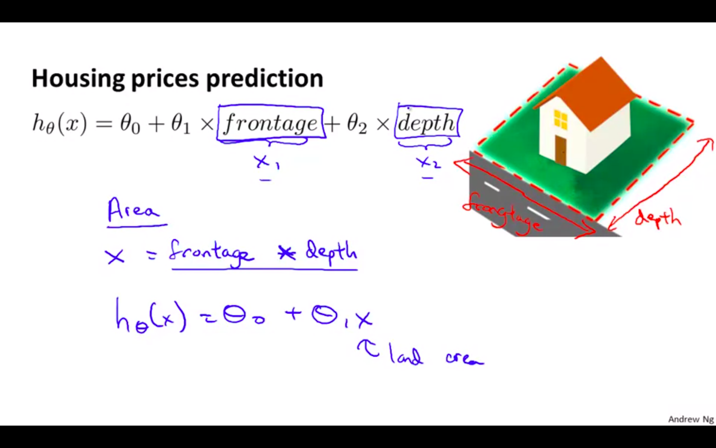
Features and Polynomial Regression

• We can improve our features and the form of our hypothesis function in a couple different ways.

• We can combine multiple features into one. For example, we can combine x-1 and x-2 into a new feature x-3 by taking x-1 * x-2.

  

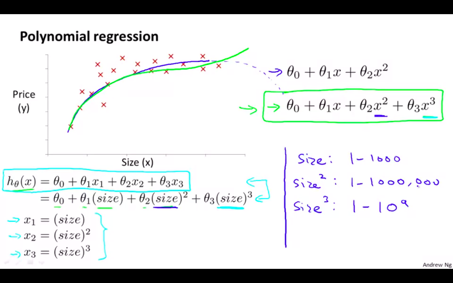
• Polynomial Regression

  • Our hypothesis function need not be linear (a straight line) if that does not fit the data well.

  • We can change the behaviour or curve of our hypothesis function by making it a quadratic, cubic or square root function (or any other form).

  • Quadratic function comes down eventually which is not applicable in this example. Prices can’t go down with increase in size of the house.

  

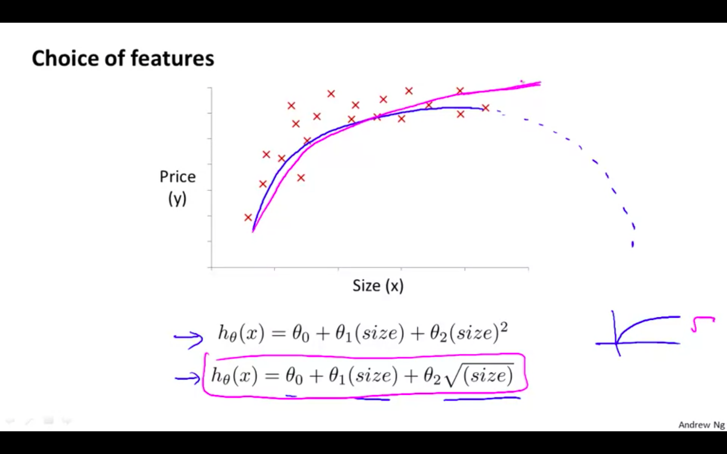
• Choice Of Features

  • One important thing to keep in mind is, if you choose your features this way then feature scaling becomes very important.

  

Computing Parameters Analytically

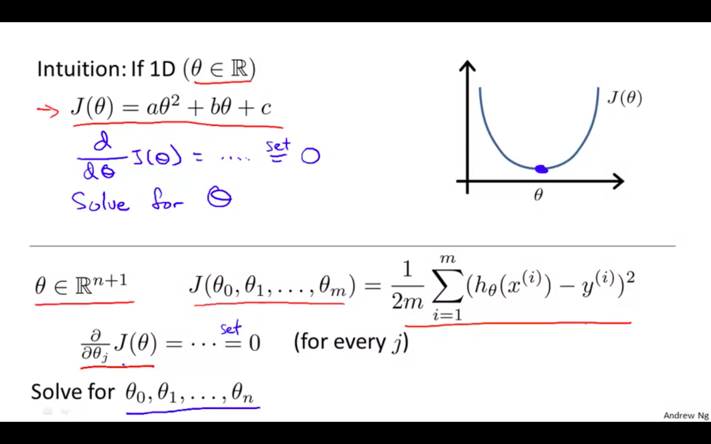
Normal Equation

• “Normal Equation” method, we will minimise J by explicitly taking its derivatives with respect to the θj ’s, and setting them to zero.

• This allows us to find the optimum theta without iteration.

• Intuition

  

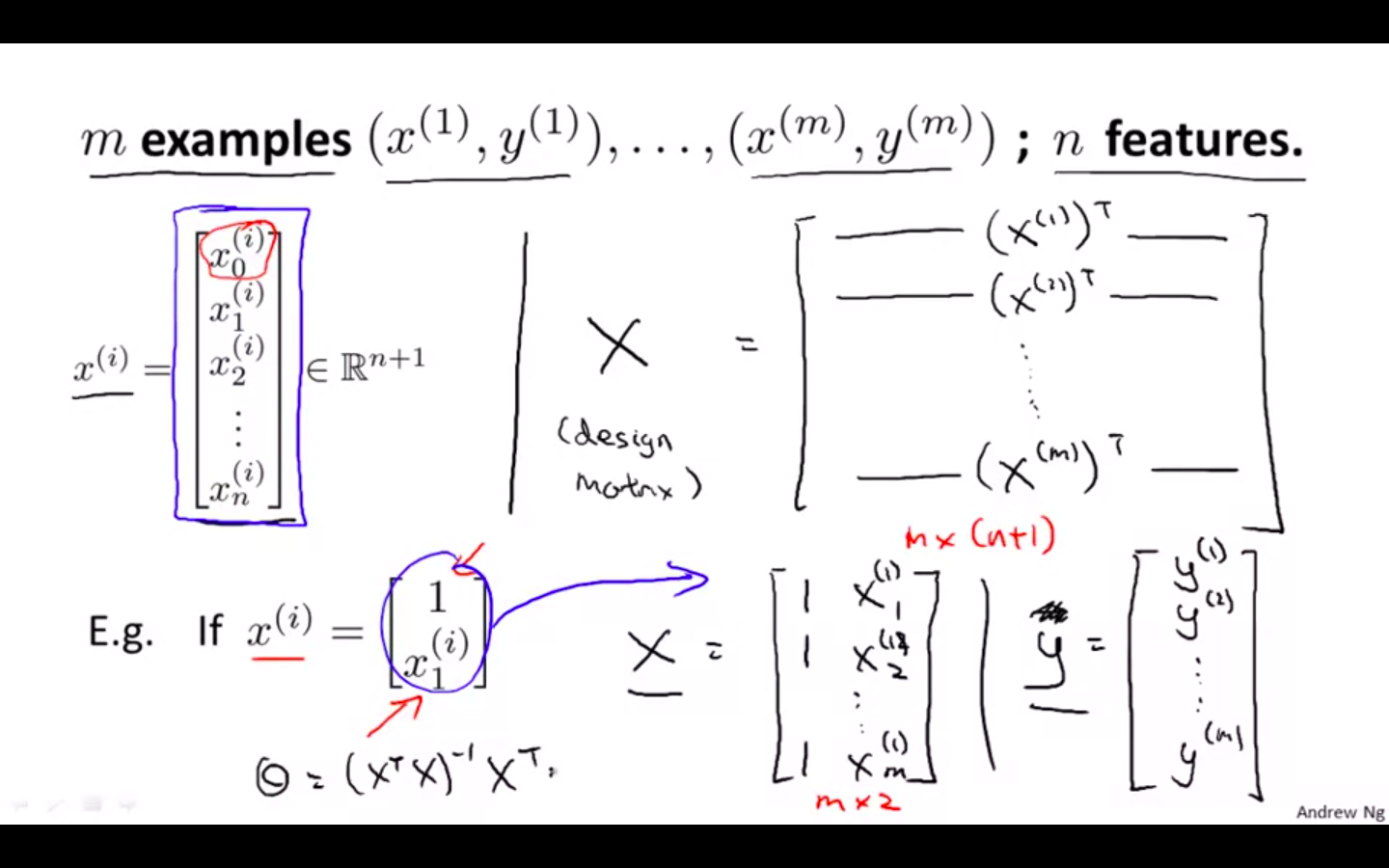
• Example

  • X - features matrix

  • y - output matrix

  

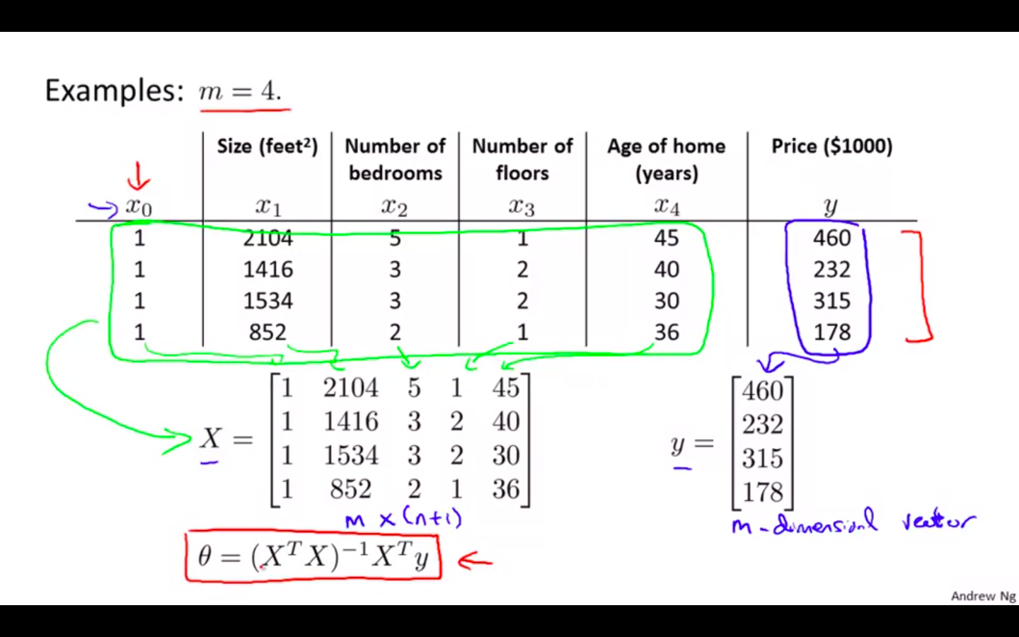
  • m examples, n features

  • X - also called as design matrix

  

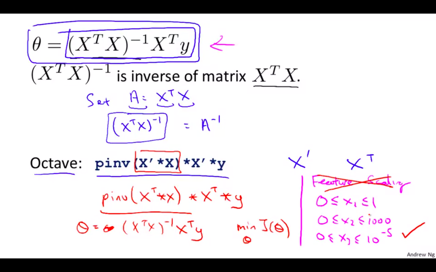
  • Feature Scaling is not needed while using normal equation method

  • Normal Equation Octave Representation

pinv( X' * X ) * X' * y

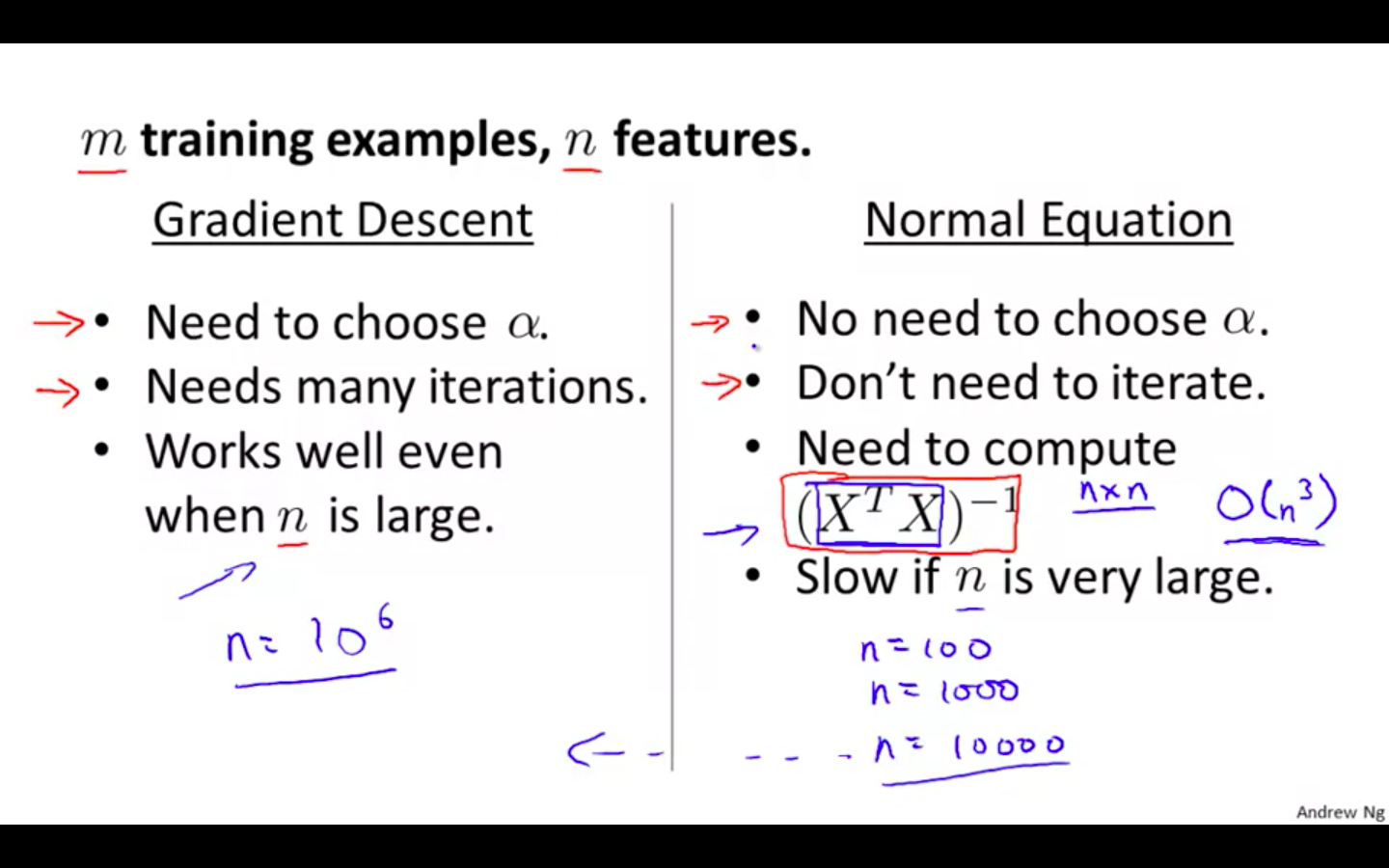
• Comparison Between Gradient Descent & Normal Equation

  • n = Normal Equation Gradient Descent

  • For some algorithms, normal equation method doesn’t work

  

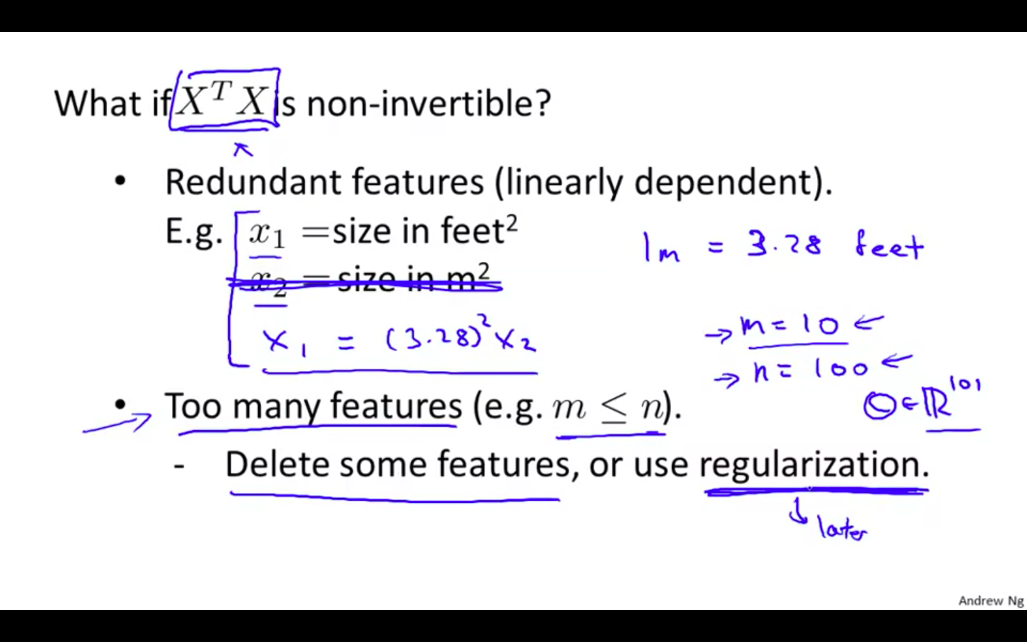
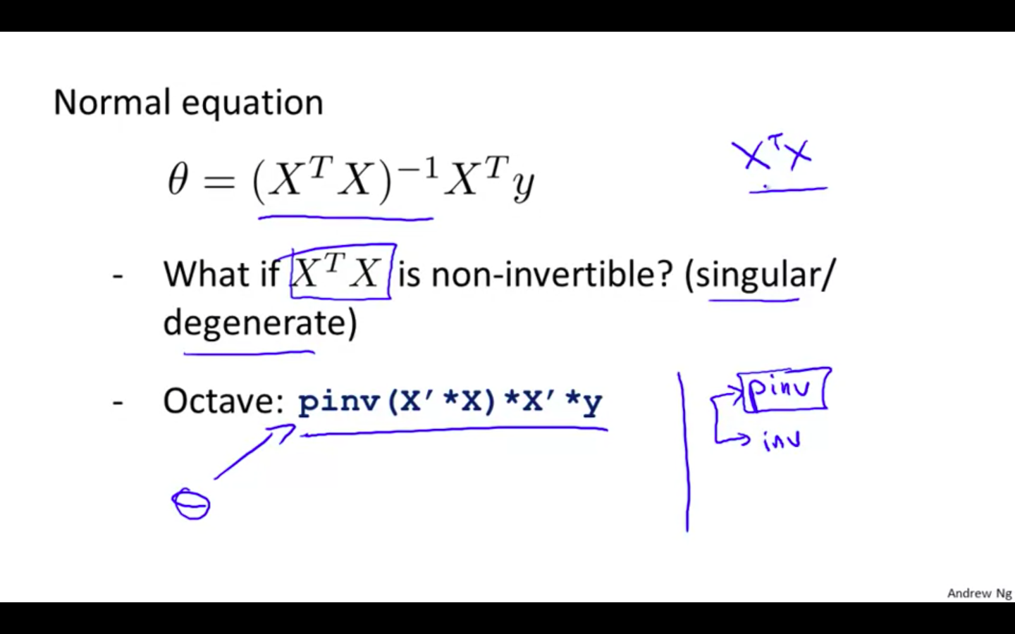
Normal Equation Noninvertibility

• When implementing the normal equation in octave we want to use the ‘pinv’ function rather than ‘inv.’ The ‘pinv’ function will give you a value of θ even if X^T * X is not invertible.

  

• Reasons for Noninvertibility

  • Redundant features, where two features are very closely related (i.e. they are linearly dependent)

  • Too many features (e.g. m ≤ n). In this case, delete some features or use “regularisation”.

• Solution

  • deleting a feature that is linearly dependent with another or deleting one or more features when there are too many features.

Lecture Presentation