Machine Learning By Andew Ng - Week 3

Classification and Representation

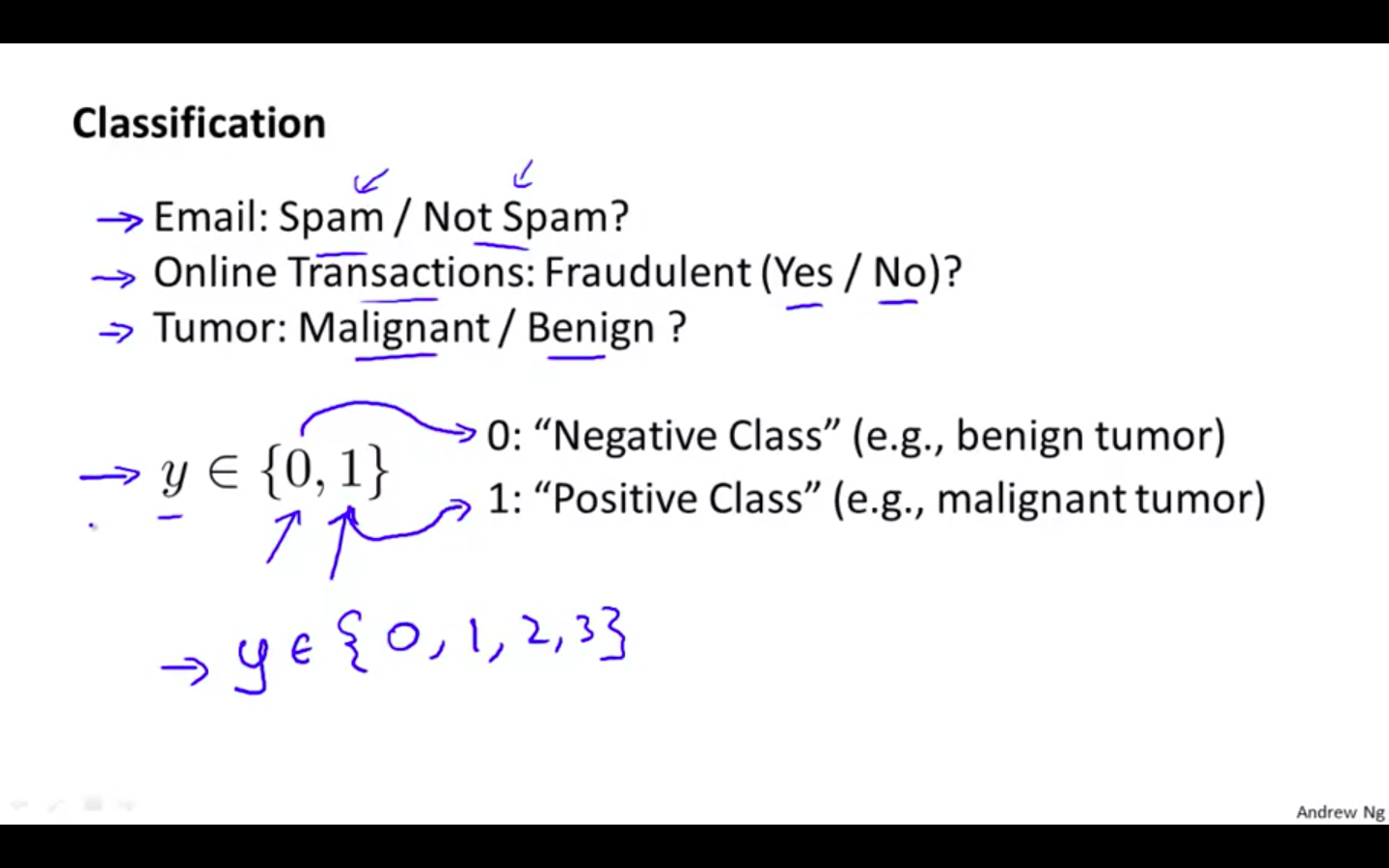
Classification

• Use Cases

  • Email: Spam / Not Spam

  • Online Transactions: Fraudulent (Yes / No )?

  • Tumor: Malignant / Benign ?

• Binary Classification

  • 0 - Negative class

    • conveys something is absent

  • 1 - Positive class

    • conveys something is present

• Example:

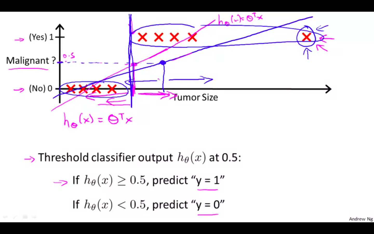
  • Applying linear regression to a classification problem is not a good idea

    • To attempt classification, one method is to use linear regression and map all predictions greater than 0.5 as a 1 and all less than 0.5 as a 0.

    • This method doesn’t work well because classification is not actually a linear function.

    

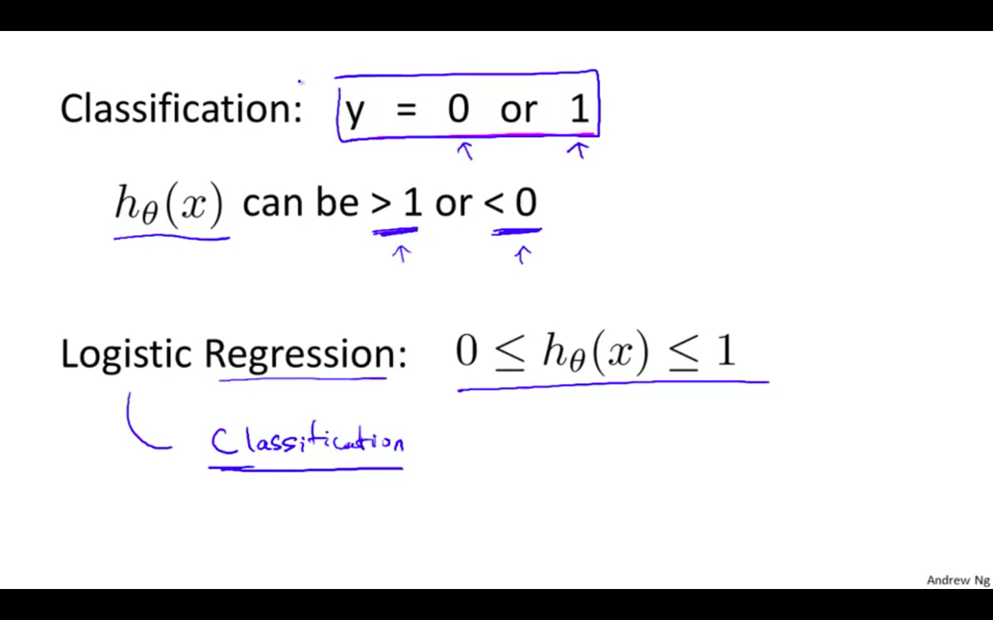
  • Classification

    • Linear regression can produce value larger than 1 or smaller than 0

    • In classification problem, label are either 1 or 0.

      • Logistic Regression: 0 ≤ h(x) ≤ 1

    

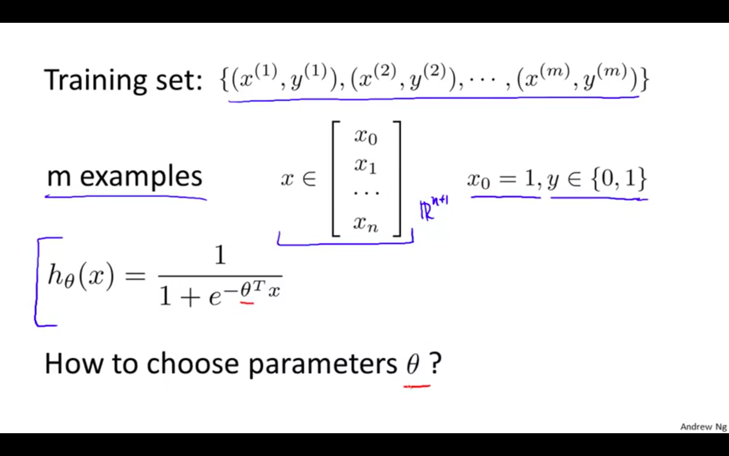
Hypothesis Representation

• Sigmoid function is zero at negative infinity and 1 at positive infinity

  • Sigmoid function == Logistic Function

  

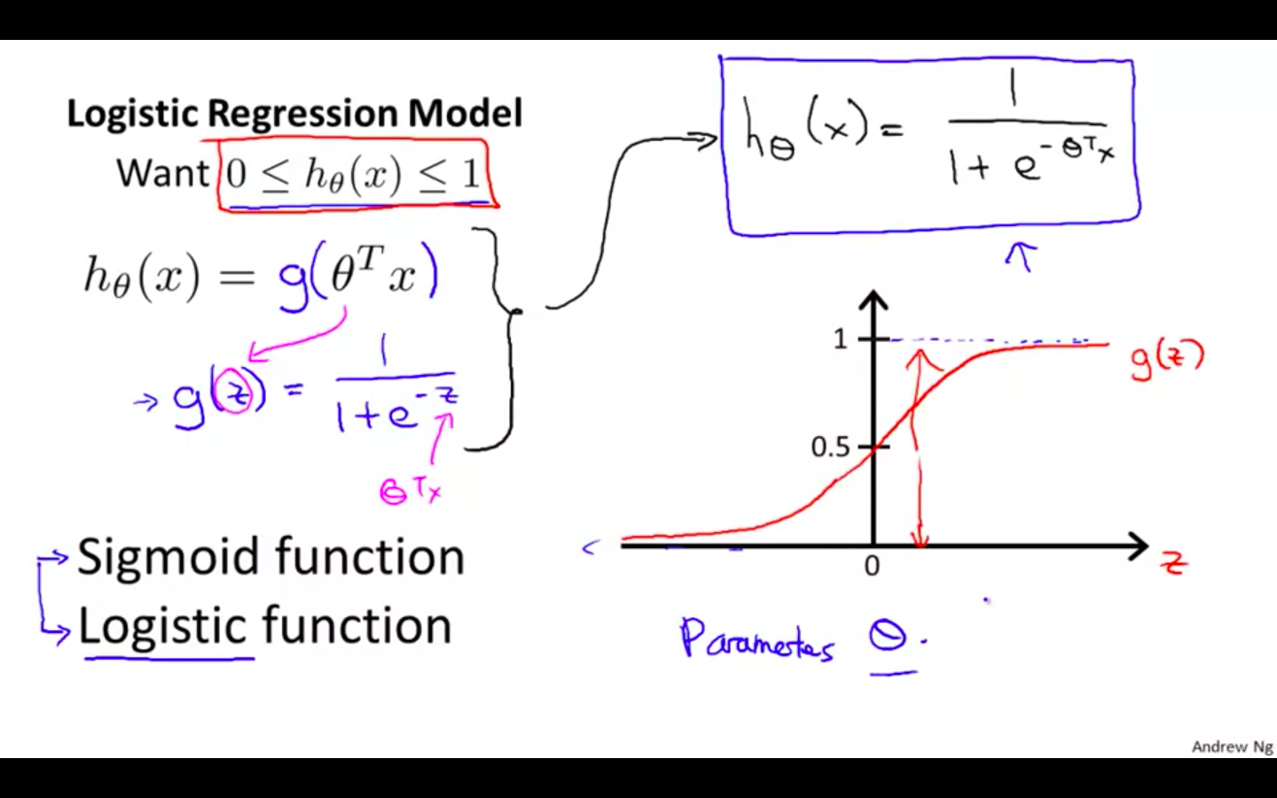
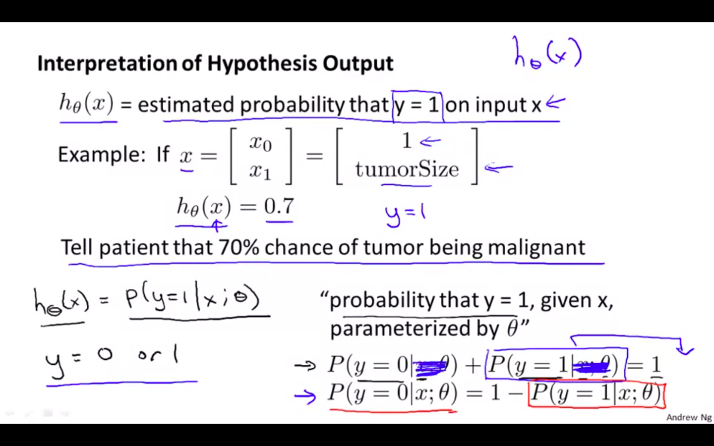
• Interpretation Of Hypothesis

  • h ( x ) = estimated probability that y = 1 on input

  

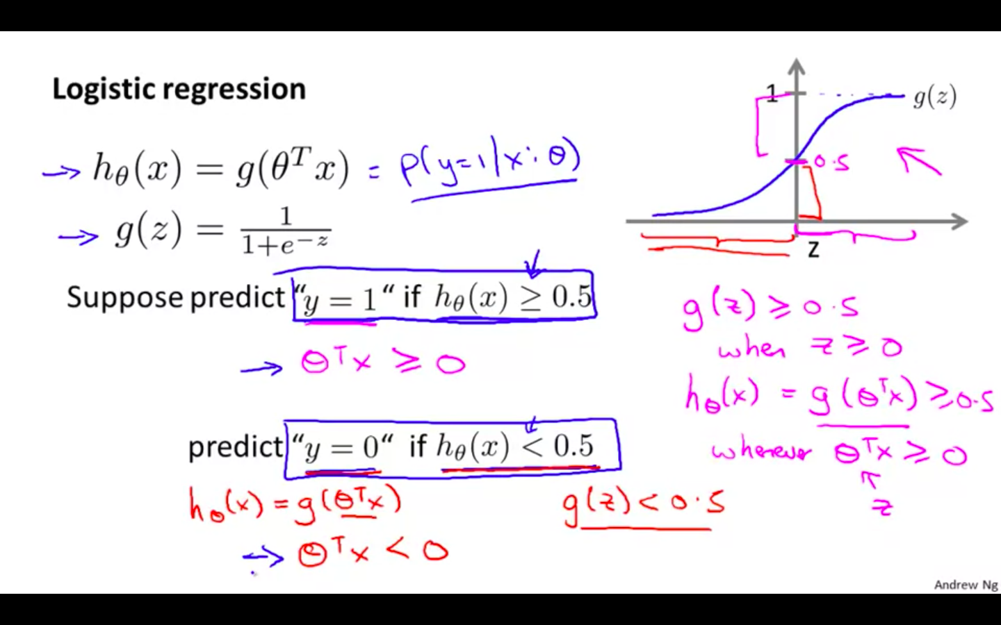
Decision Boundary

• Predict y = 1

  • h ( x ) ≥ 0.5 : y = 1

  • thetha^T X ≥ 0

• Predict y = 0

  • h ( x )

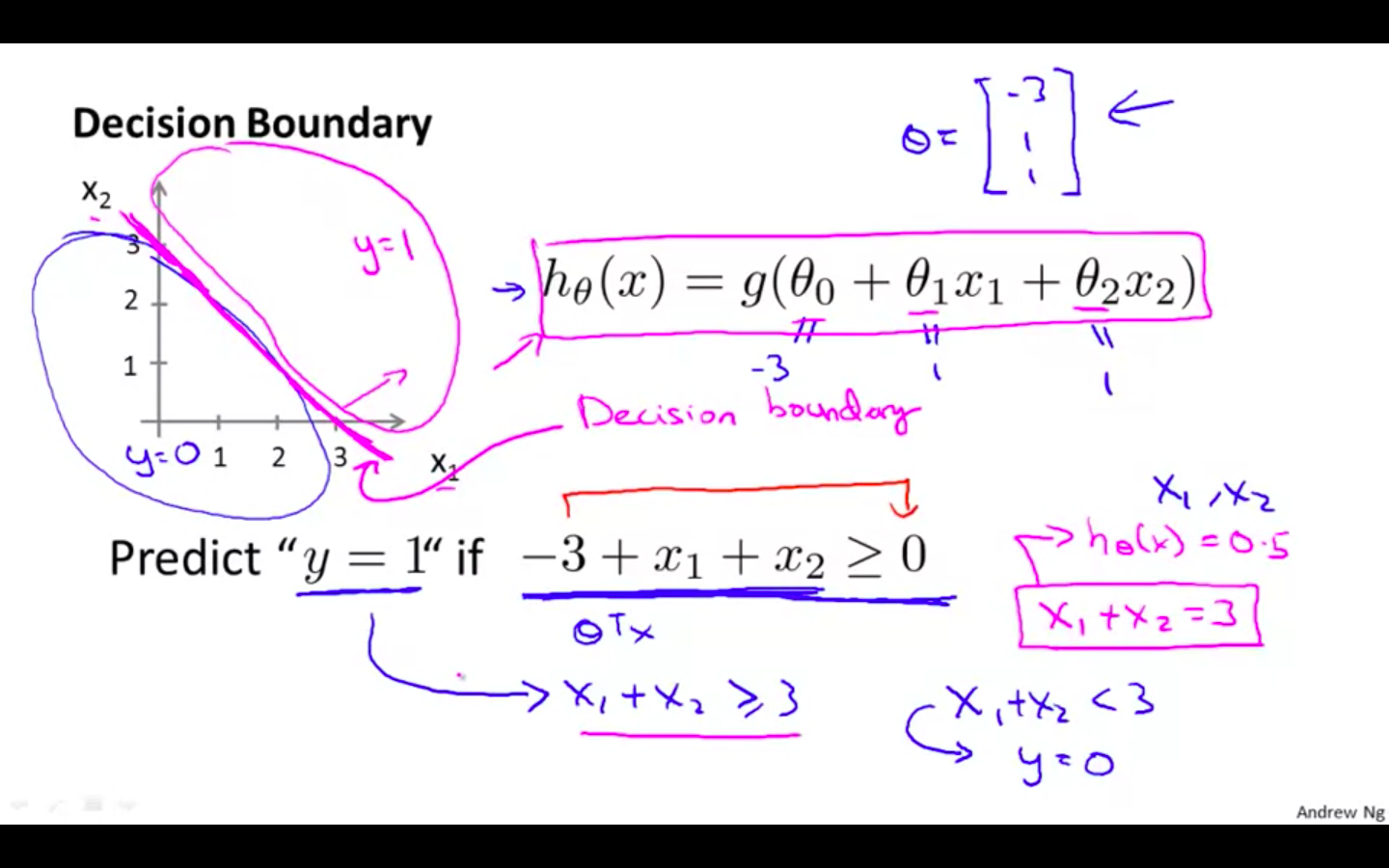
• Decision boundary

  • The decision boundary is the line that separates the area where y = 0 and where y = 1.

  • It is created by our hypothesis function.

  • This is the property of the hypothesis and not of the data

  

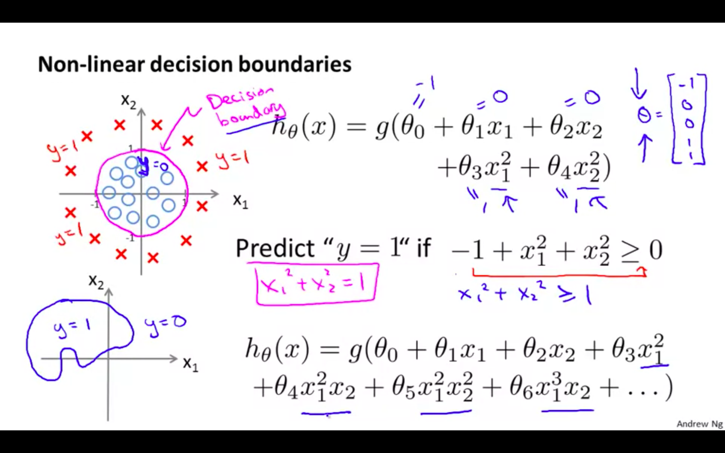
  • Non Linear Decision Boundary

    • Decision Boundary doesn’t need to be linear

    • High order polynomials can also be resulted in a complex decision boundary

    

Logistic Regression Model

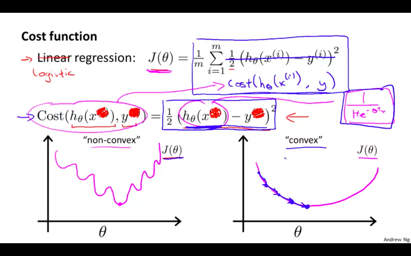
Cost Function

• Concept

  

• We cannot use the same cost function that we use for linear regression because the Logistic Function will cause the output to be wavy, causing many local optima.

• In other words, it will not be a convex function.

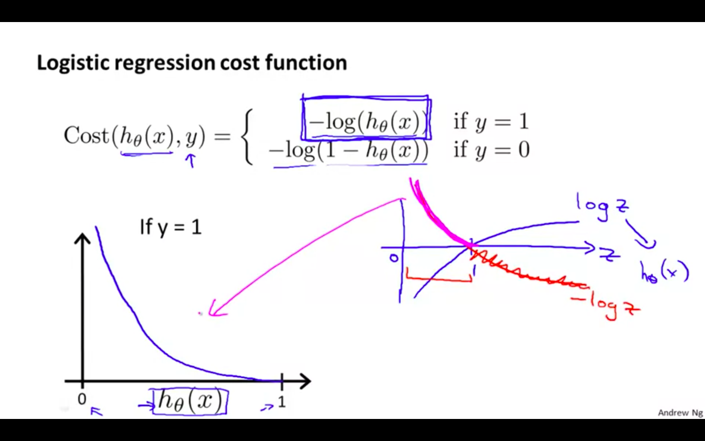
• Case 1

  • When y = 1, we get the following plot for J (theta) vs h ( x )

    • If our correct answer ‘y’ is 1, then the cost function will be 0 if our hypothesis function outputs 1.

    • If our hypothesis approaches 0, then the cost function will approach infinity.

    

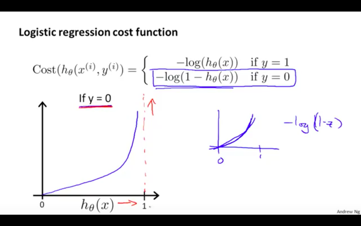
• Case 2

  • When y = 0, we get the following plot for J (theta) vs h ( x )

    • If our correct answer ‘y’ is 0, then the cost function will be 0 if our hypothesis function also outputs 0.

    • If our hypothesis approaches 1, then the cost function will approach infinity.

    

• Note that writing the cost function in this way guarantees that J(θ) is convex for logistic regression.

Simplified Cost Function and Gradient Descent

• Modified Cost Function ( Simple )

  • Compress our cost function’s two conditional cases into one case:

  

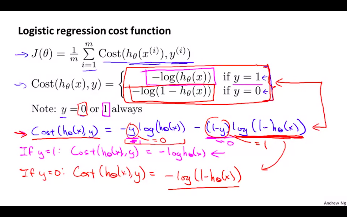
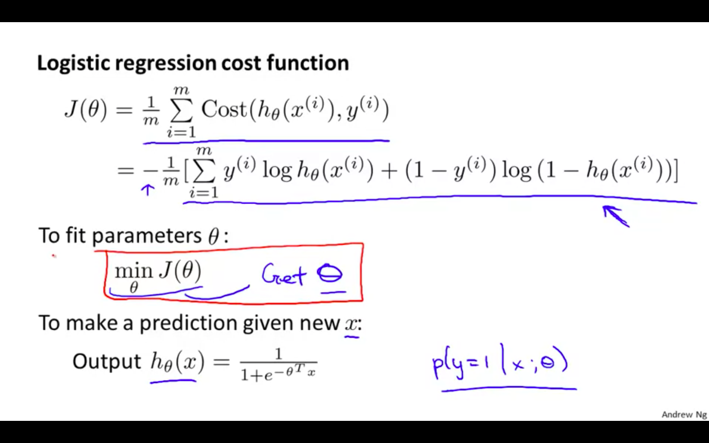
  • We can fully write out our entire cost function as follows:

  

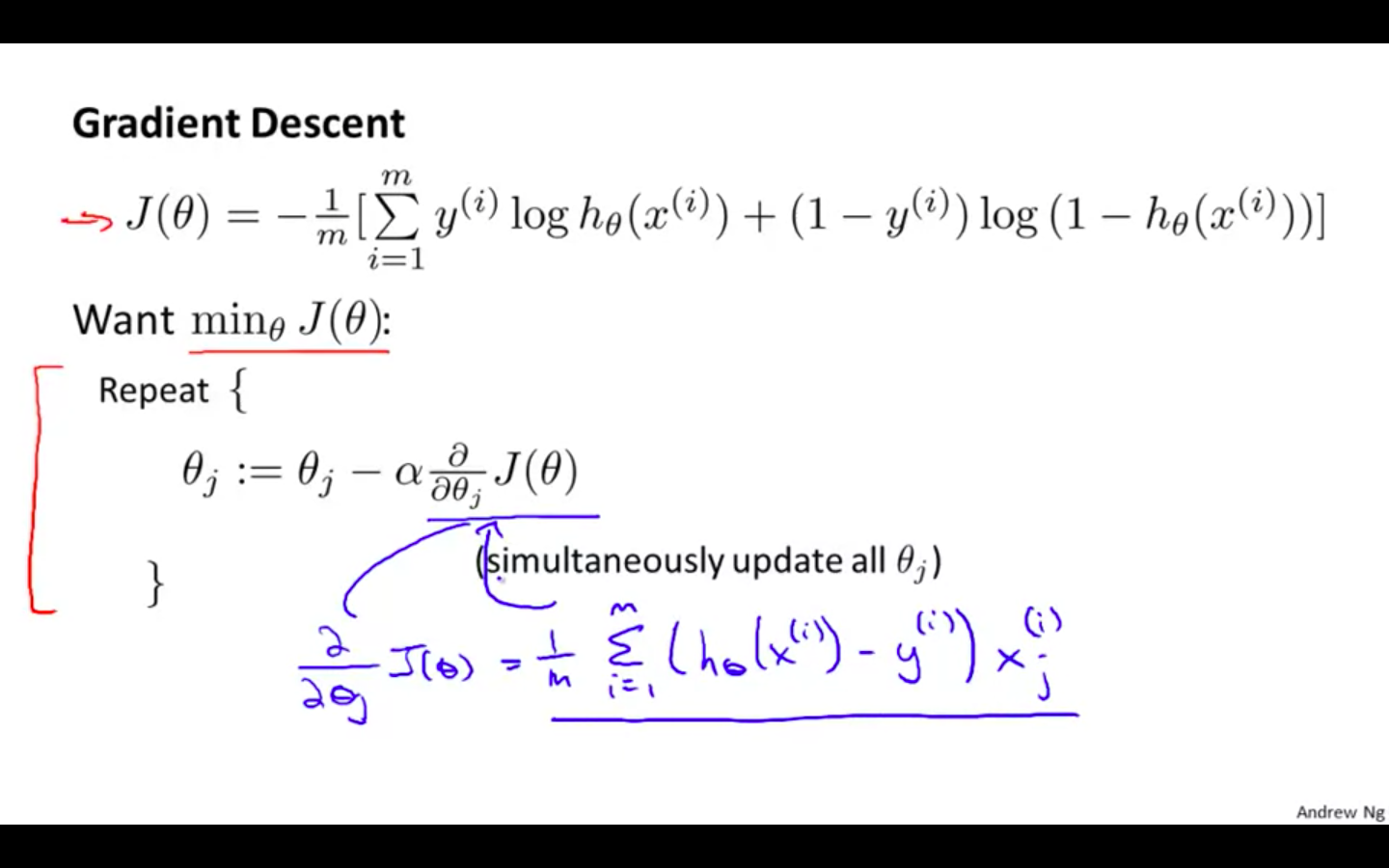
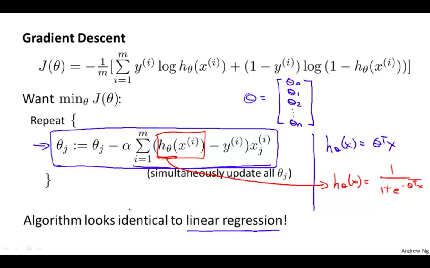
• Gradient Descent

  • Notice that this algorithm is identical to the one we used in linear regression.

  • We still have to simultaneously update all values in theta.

  

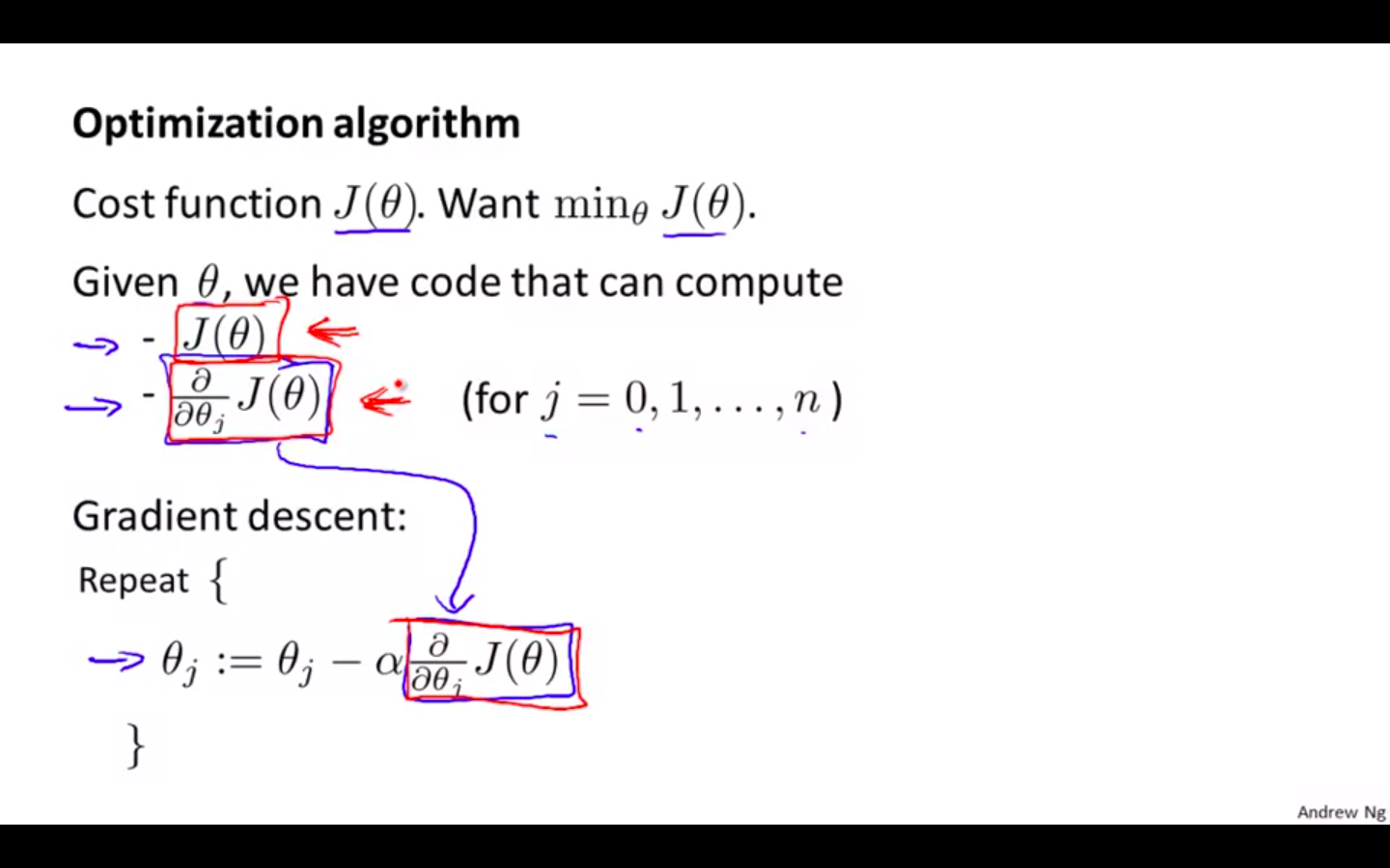
Advanced Optimisation

• Optimisation Algorithm

  • Minimising the cost function as efficient as possible

  

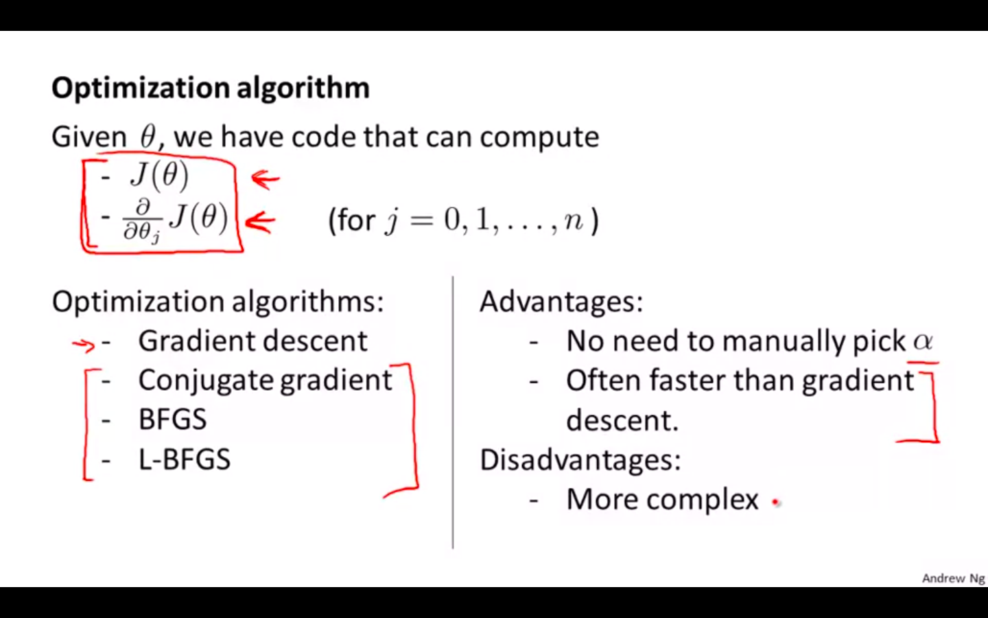
• Advance Optimisation Algorithms

  • Algorithms

    • Gradient Descent

    • Conjugate Gradient

    • BFGS

    • L-BFGS

  • Advantages

    • No need to manually pick alpha

    • Often faster than gradient descent

  • Disadvantage

    • More complex

  

• Example 1

  • Implementing function minimisation unconstrained

    • fminunc() in octave programming

  

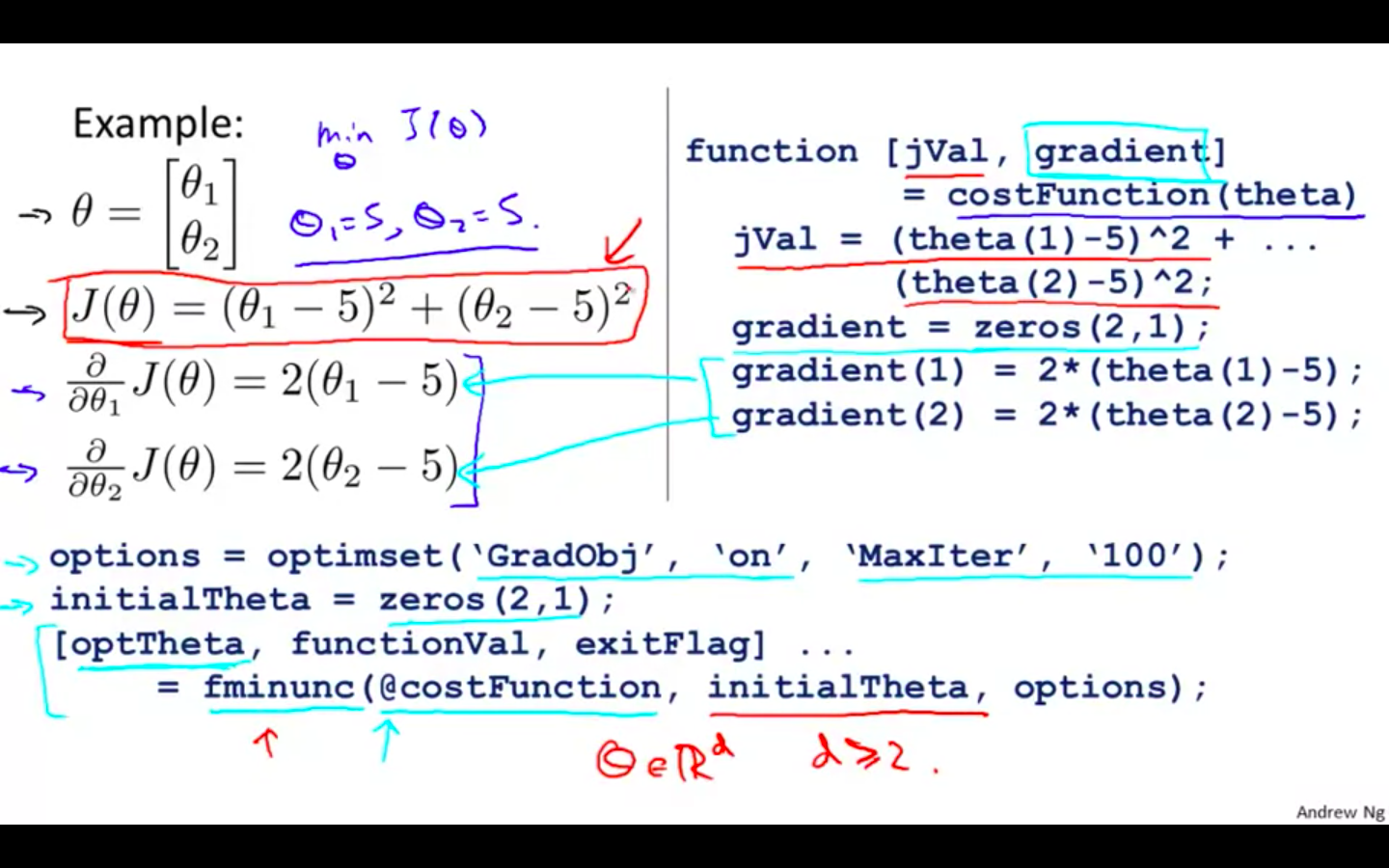
• Example 2

  

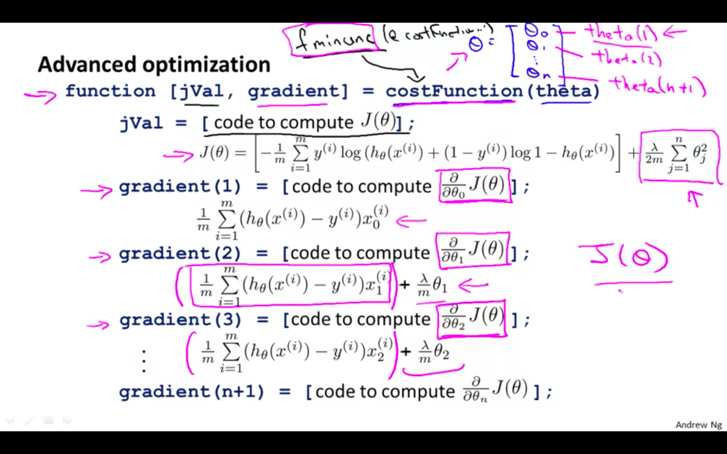
• Octave / Matlab Snippets

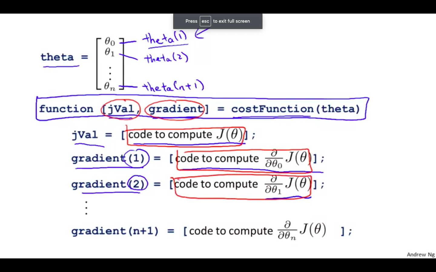
  • We can write a single function that returns both of these

function [jVal, gradient] = costFunction(theta)
  jVal = [...code to compute J(theta)...];
  gradient = [...code to compute derivative of J(theta)...];
end

- Then we can use octave's "fminunc()" optimization algorithm along with the "optimset()" function that creates an object containing the options we want to send to "fminunc()".

- We give to the function "fminunc()" our cost function, our initial vector of theta values, and the "options" object that we created beforehand.

options = optimset('GradObj', 'on', 'MaxIter', 100);
initialTheta = zeros(2,1);
   [optTheta, functionVal, exitFlag] = fminunc(@costFunction, initialTheta, options);

Multi-class Classification

Multi-class Classification: One-vs-all

• Instead of y = {0,1} we will expand our definition so that y = {0,1…n}.

• Since y = {0,1…n}, we divide our problem into n+1 (+1 because the index starts at 0) binary classification problems; in each one, we predict the probability that ‘y’ is a member of one of our classes

• Use Cases

  • Email sorting / tagging : Work, Family, Friends, Hobby

  • Medical diagrams: Not ill, Cold, Flu

  • Weather: Sunny, Cloud, Rain, Snow

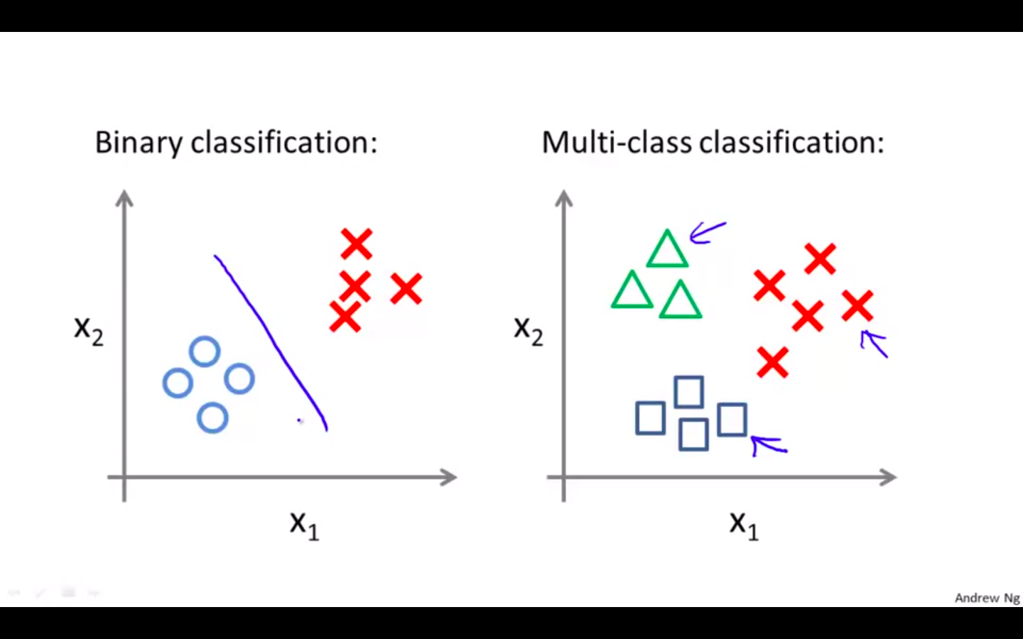
• Difference in data visualisation in binary classification and multi-class classification

  

• One vs All Algorithm

  • It chooses as first class and other classes as second class and does the Binary logistic regression among them.

  • It changes the active class and repeats until all the classes have been covered as the active class.

  

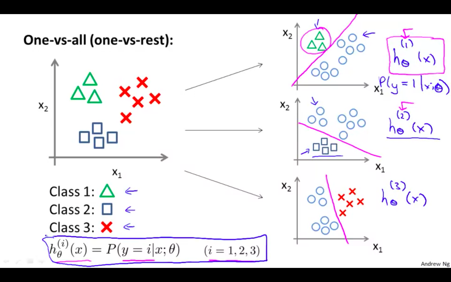
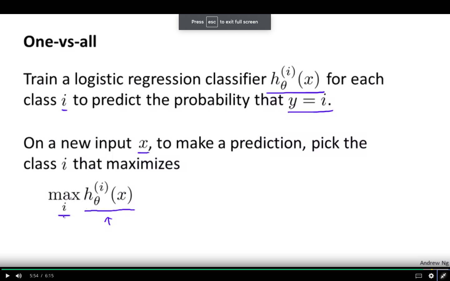
• Using the algorithm

  • Select the i for which the hypothesis is the maximum as the prediction

  

Solving the Problem of Overfitting

The Problem of Overfitting

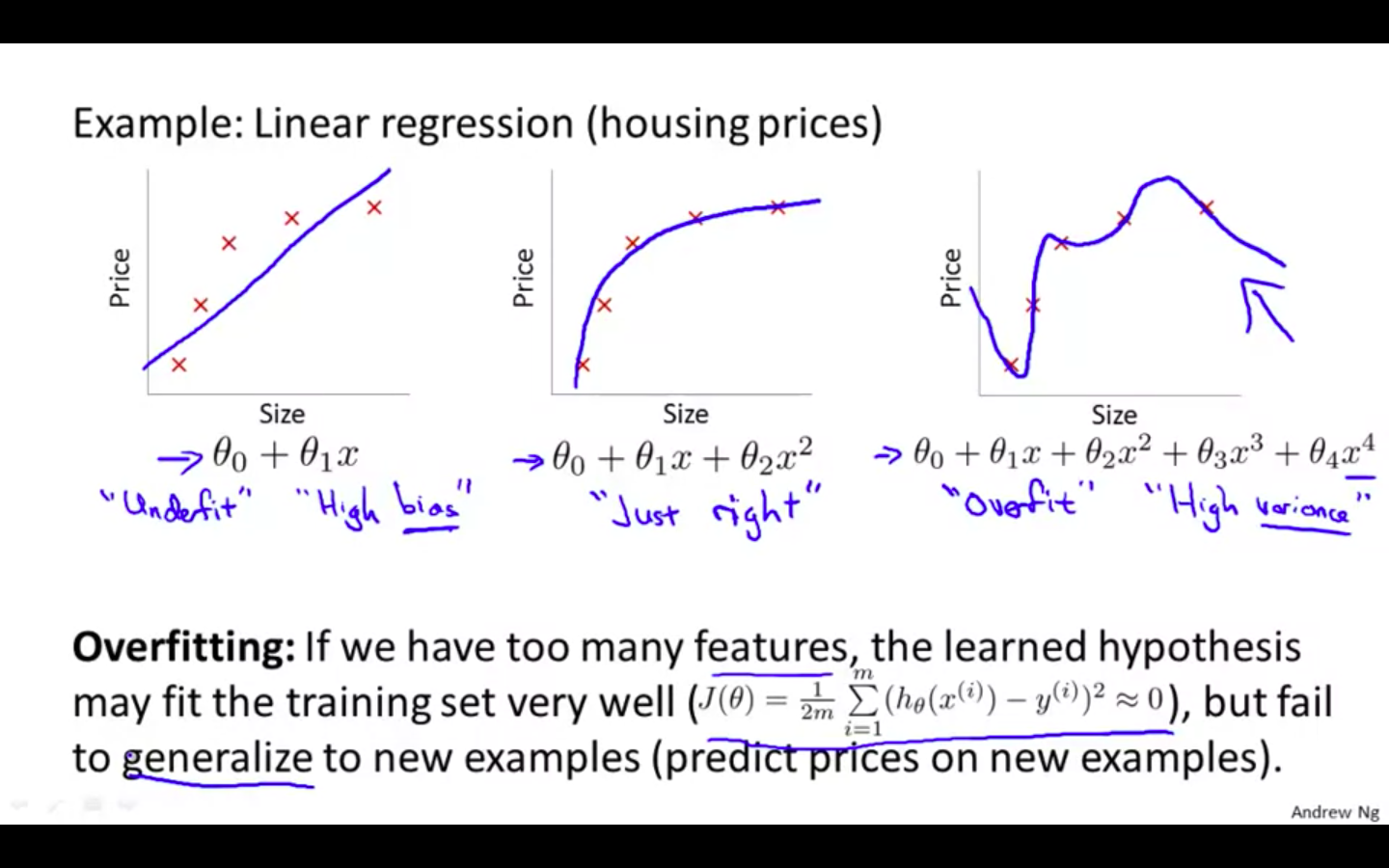
• If we have too many features, the learned hypothesis may fit the training set very well ( where cost function is similar to equal to 0 ), but fail to generalise to new examples ( predict prices on new examples )

• Underfit or High bias

  • Underfitting, or high bias, is when the form of our hypothesis function h maps poorly to the trend of the data.

  • It is usually caused by a function that is too simple or uses too few features.

• Overfit or High Variance

  • Overfitting, or high variance, is caused by a hypothesis function that fits the available data but does not generalize well to predict new data.

  • It is usually caused by a complicated function that creates a lot of unnecessary curves and angles unrelated to the data.

• Overfitting in Linear Regression

  

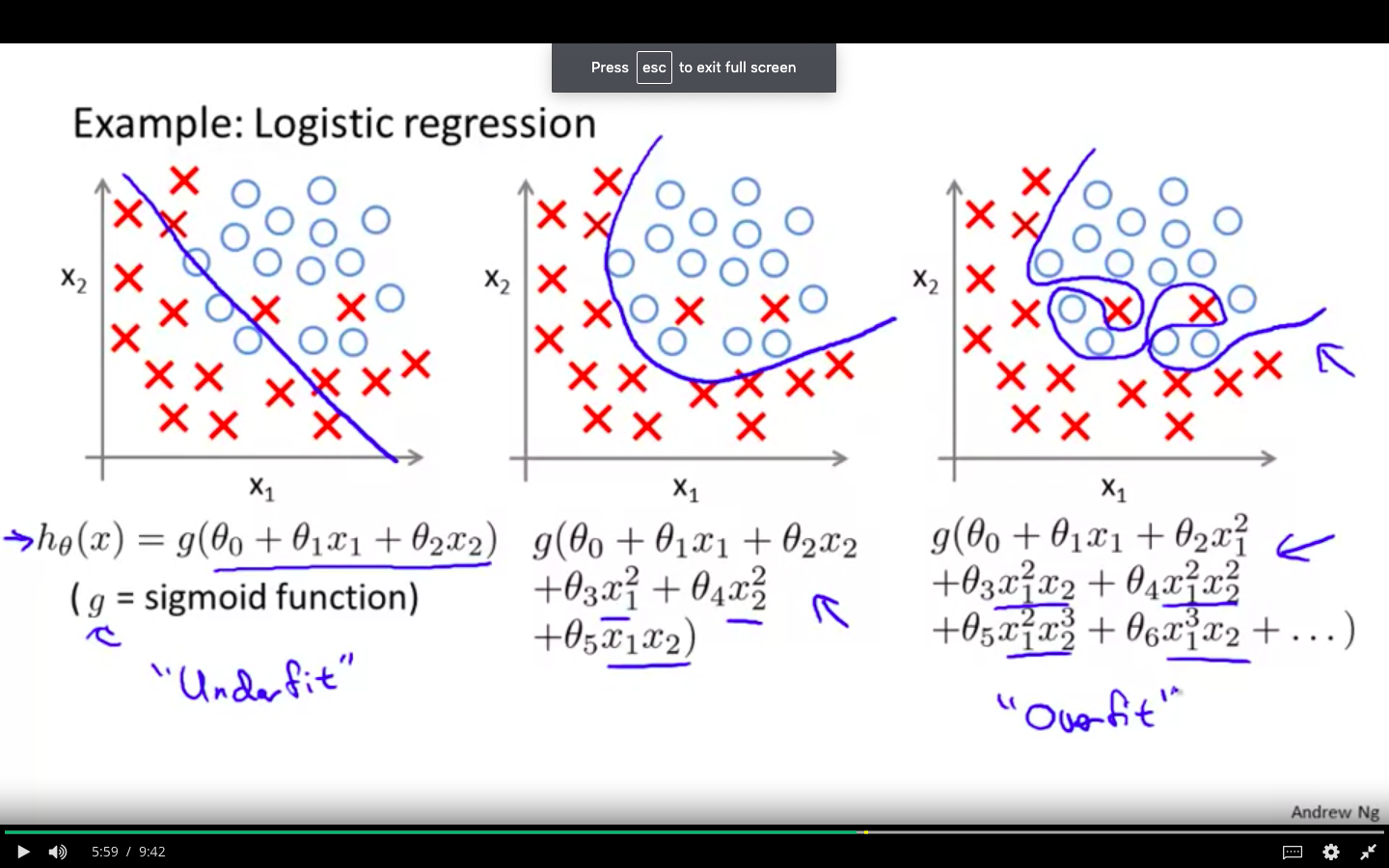
• Overfitting in Logistic Regression

  

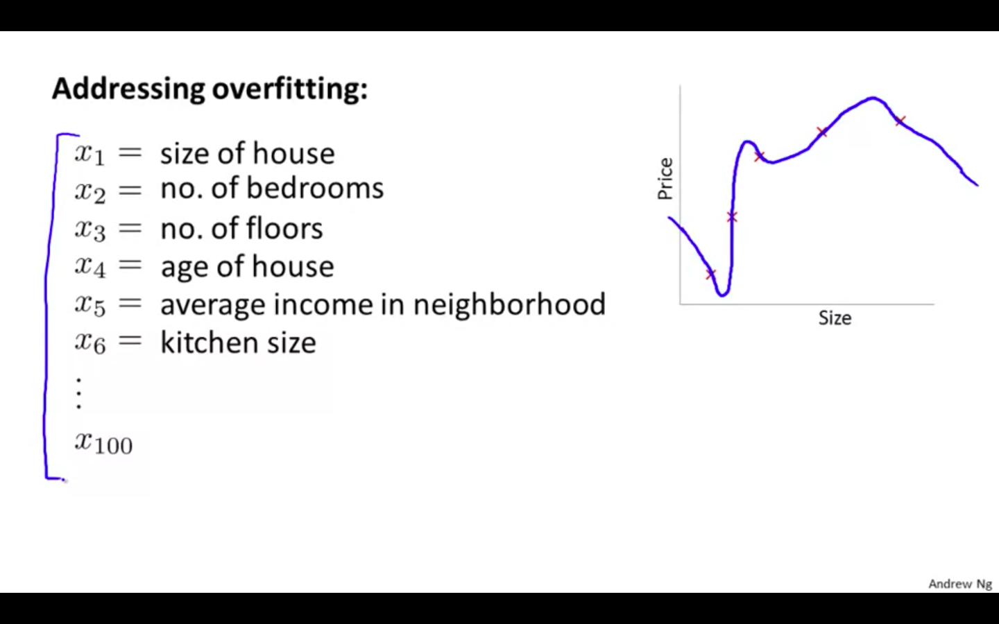
• Causes of Overfitting

  • Too many features & Small dataset

  

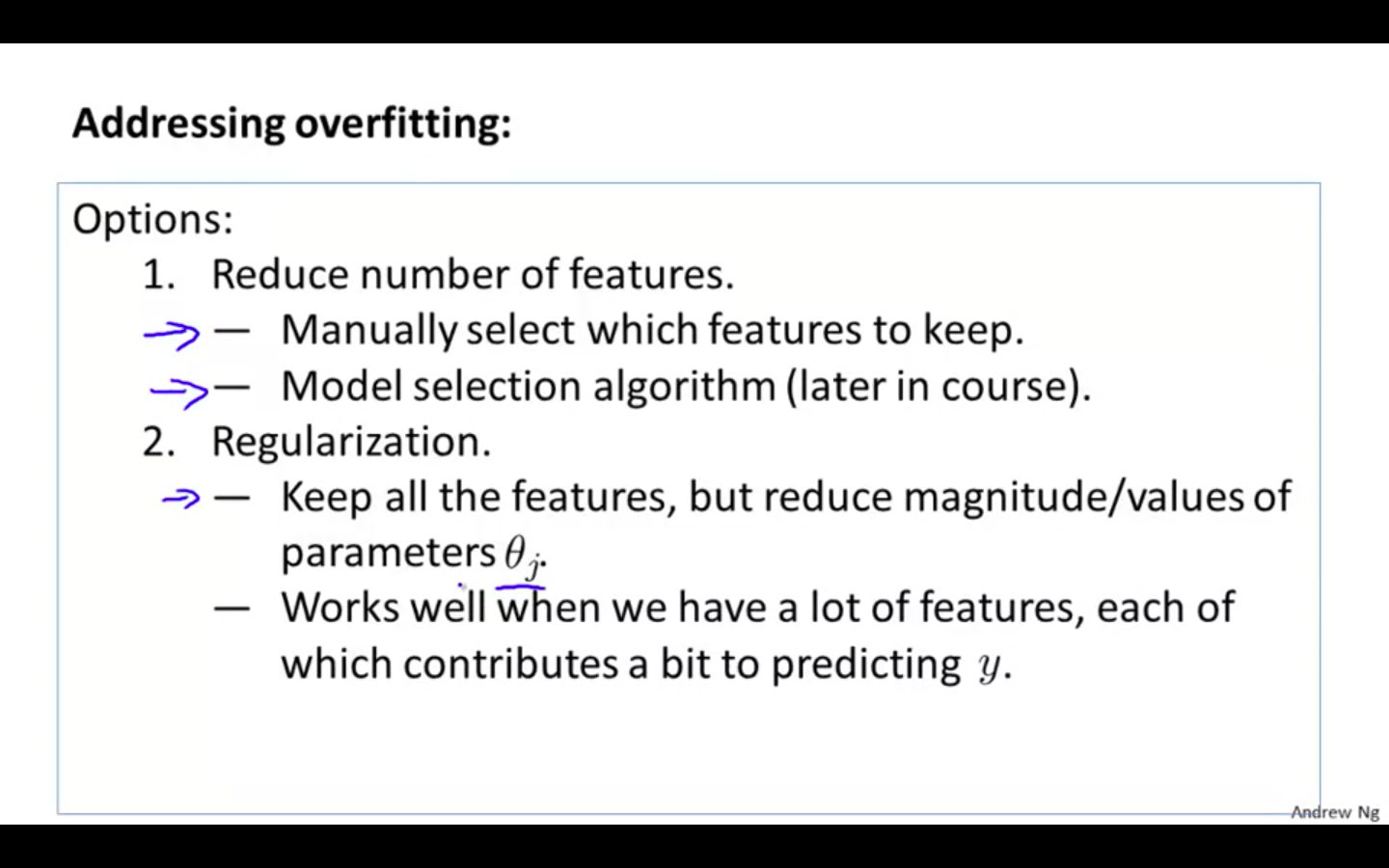
• Solution to Overfitting

  • Reduce number of features

    • Manually select which features to keep

    • Model selection algorithm

  • Regularisation

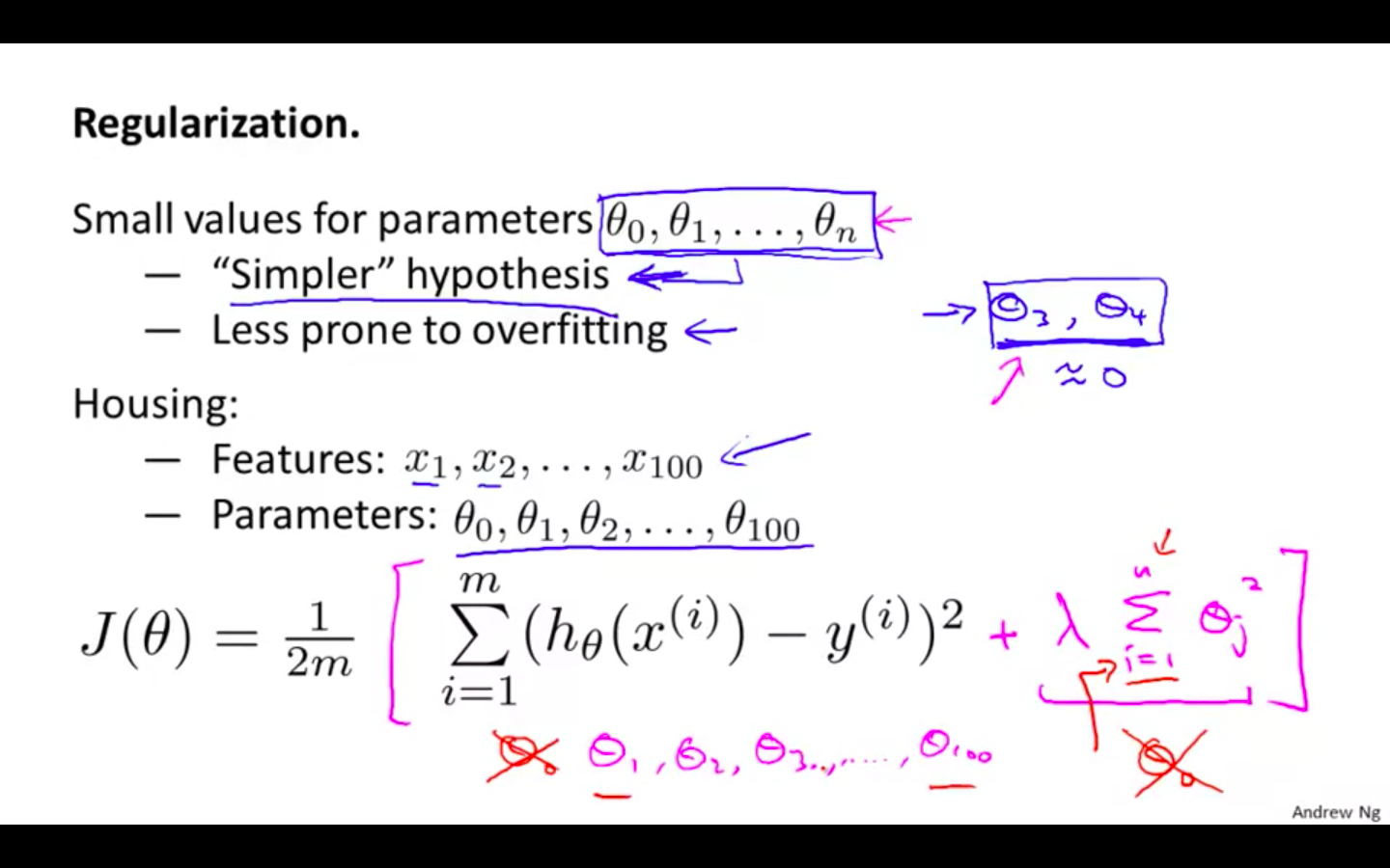
    • Keep all the features, but reduce magnitude / values of parameters

    • Works well when we have a lot of features, each of which contributes a bit to predicting y.

  

Cost Function

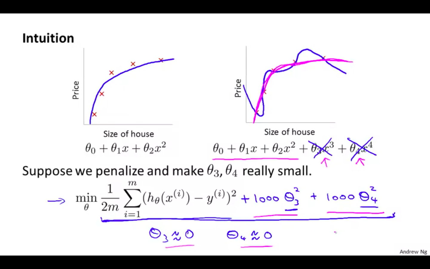
• Intuition

  • If we have overfitting from our hypothesis function, we can reduce the weight that some of the terms in our function carry by increasing their cost.

  • Without actually getting rid of these features or changing the form of our hypothesis, we can instead modify our cost function:

  • If we reduce the features to near zero, will result in slight change in hypothesis

  • New hypothesis will fits the data better due to extra small terms

  

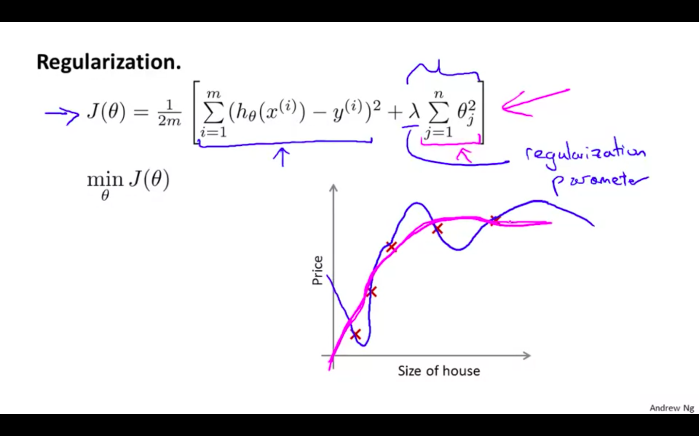
• Regularisation

  • The λ, or lambda, is the regularization parameter.

  • It determines how much the costs of our theta parameters are inflated.

  

• Example

  

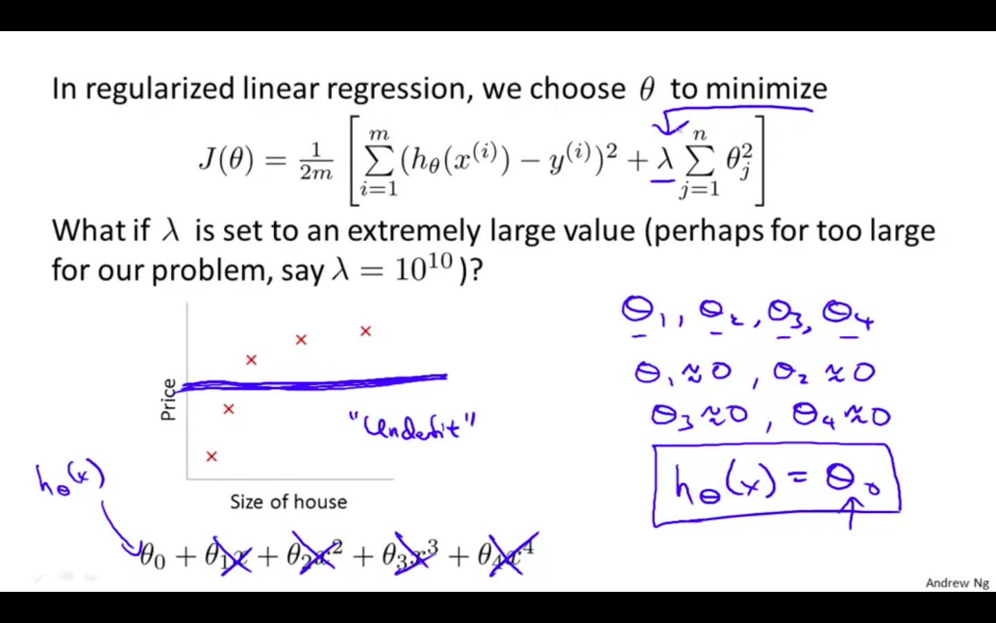
• Regularisation Parameter

  • If lambda is chosen to be too large, it may smooth out the function too much and cause underfitting.

  

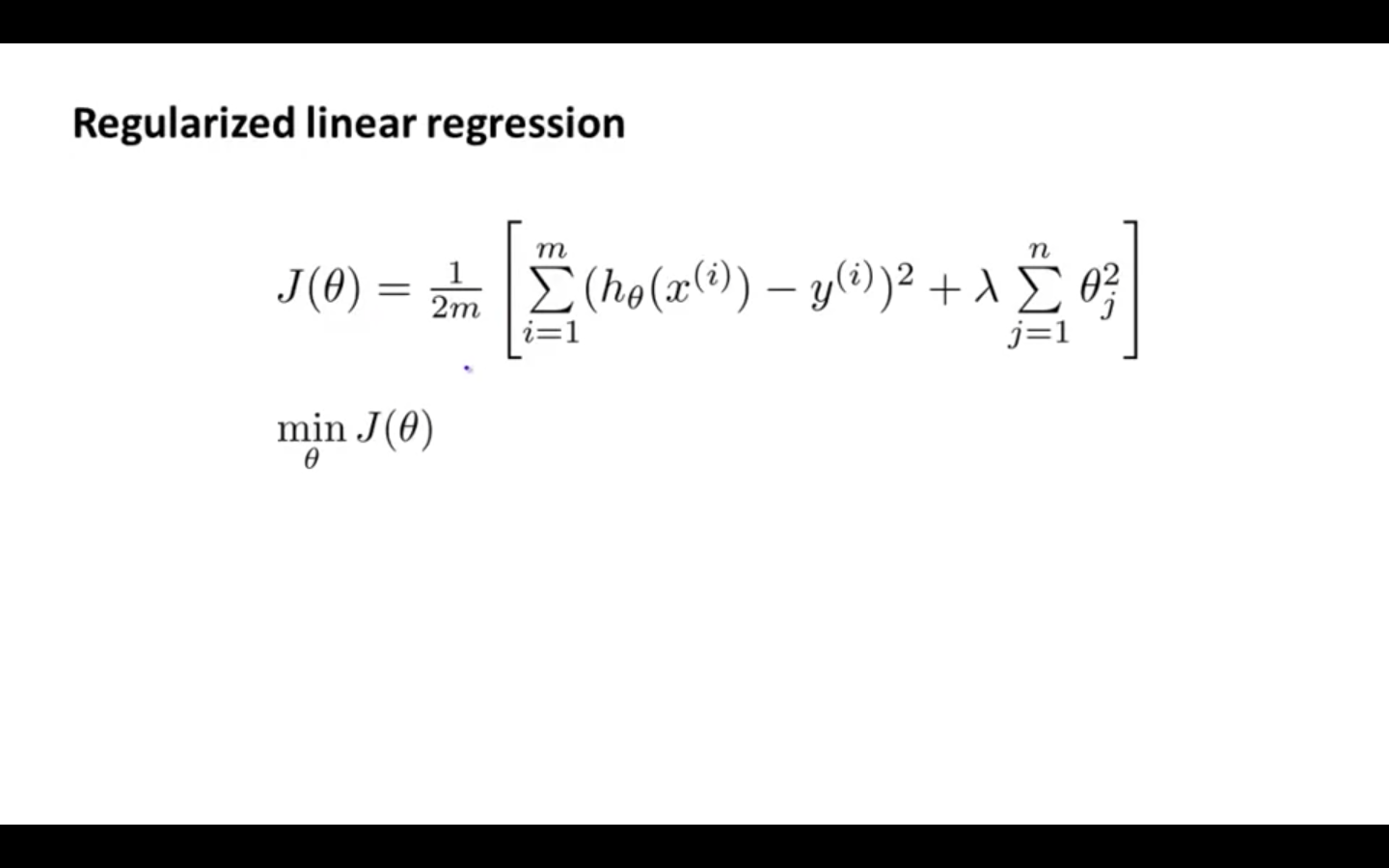
Regularised Linear Regression

• Regularised Linear Regression

  

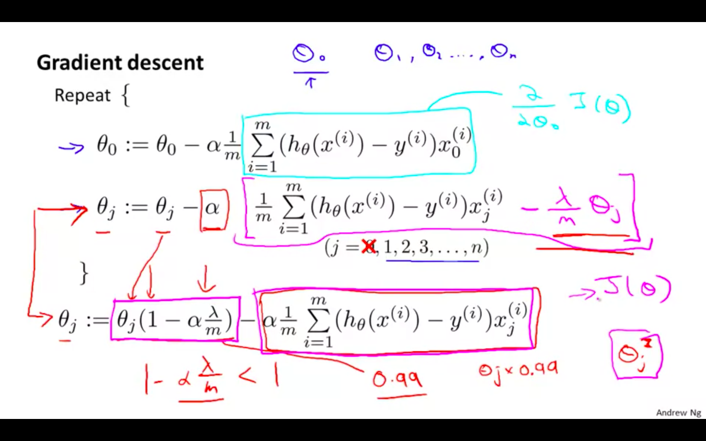
• Regularised Gradient Descent

  • We will modify our gradient descent function to separate out theta_0 from the rest of the parameters because we do not want to penalise theta_0

  • Intuitively you can see it as reducing the value of theta_j​ by some amount on every update.

  • Notice that the second term is now exactly the same as it was before.

  • theta_0 is not regularised

  

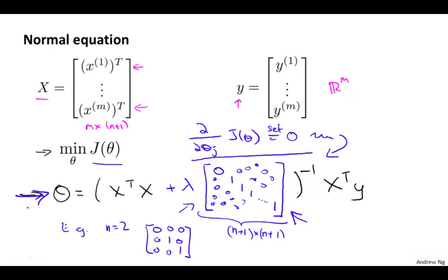
• Regularised Normal Equation

  • To add in regularisation, the equation is the same as our original, except that we add another term inside the parentheses:

  

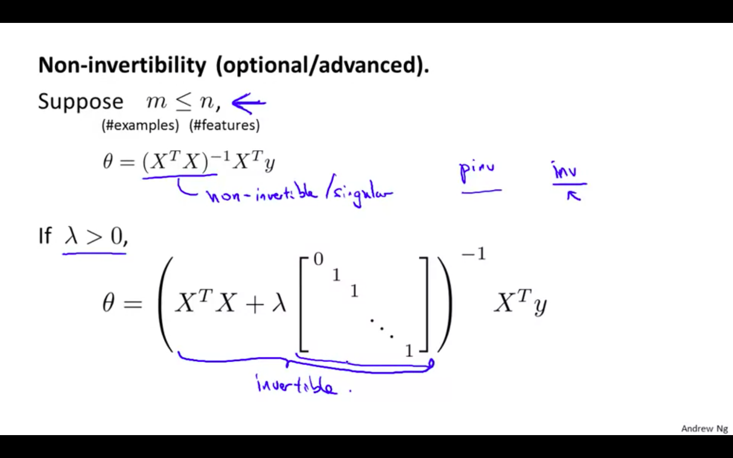
• Regularisation in Non-Invertibility

  • Recall that if m < n, then X^T _ X is non-invertible. However, when we add the term λ⋅L, then X^T _ X + λ⋅L becomes invertible.

Regularised Logistic Regression

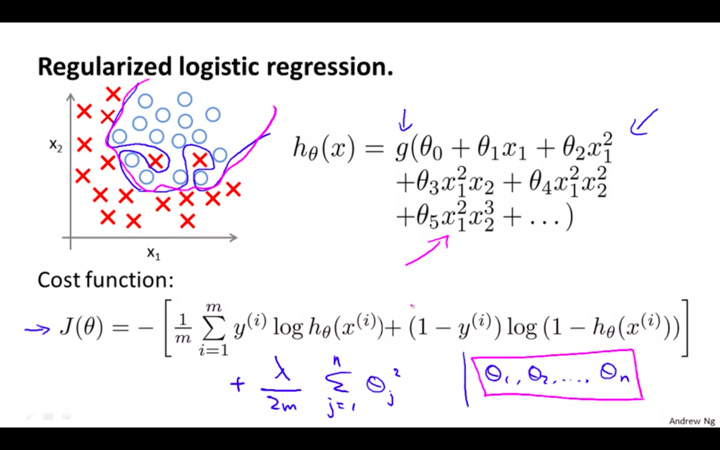
• Regularised Logistic Regression

  • image shows how the regularised function, displayed by the pink line, is less likely to overfit than the non-regularised function represented by the blue line:

  • We can regularise this equation by adding a term to the end

  

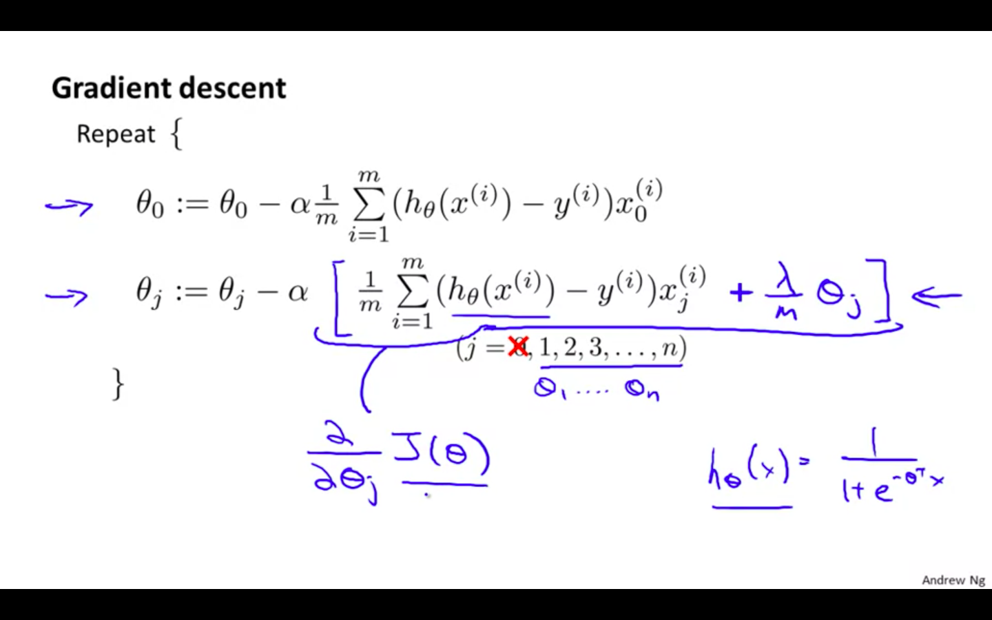
• Regularised Gradient Descent

  • Equation seems identical with regularised gradient descent of linear regression

    • Hypothesis is different in both regression

  • theta_0 is not regularised

  • computing the equation, we should continuously update the two following equations:

  

• Regularised Advanced Optimisation

  

Lecture Presentation