Machine Learning By Andew Ng - Week 5

Cost Function and Backpropagation

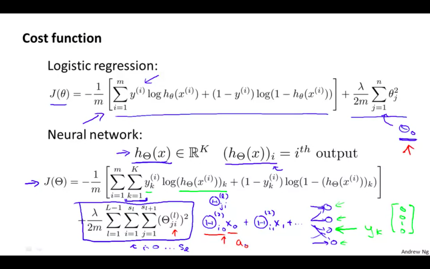
Cost Function

• Let’s first define a few variables that we will need to use:

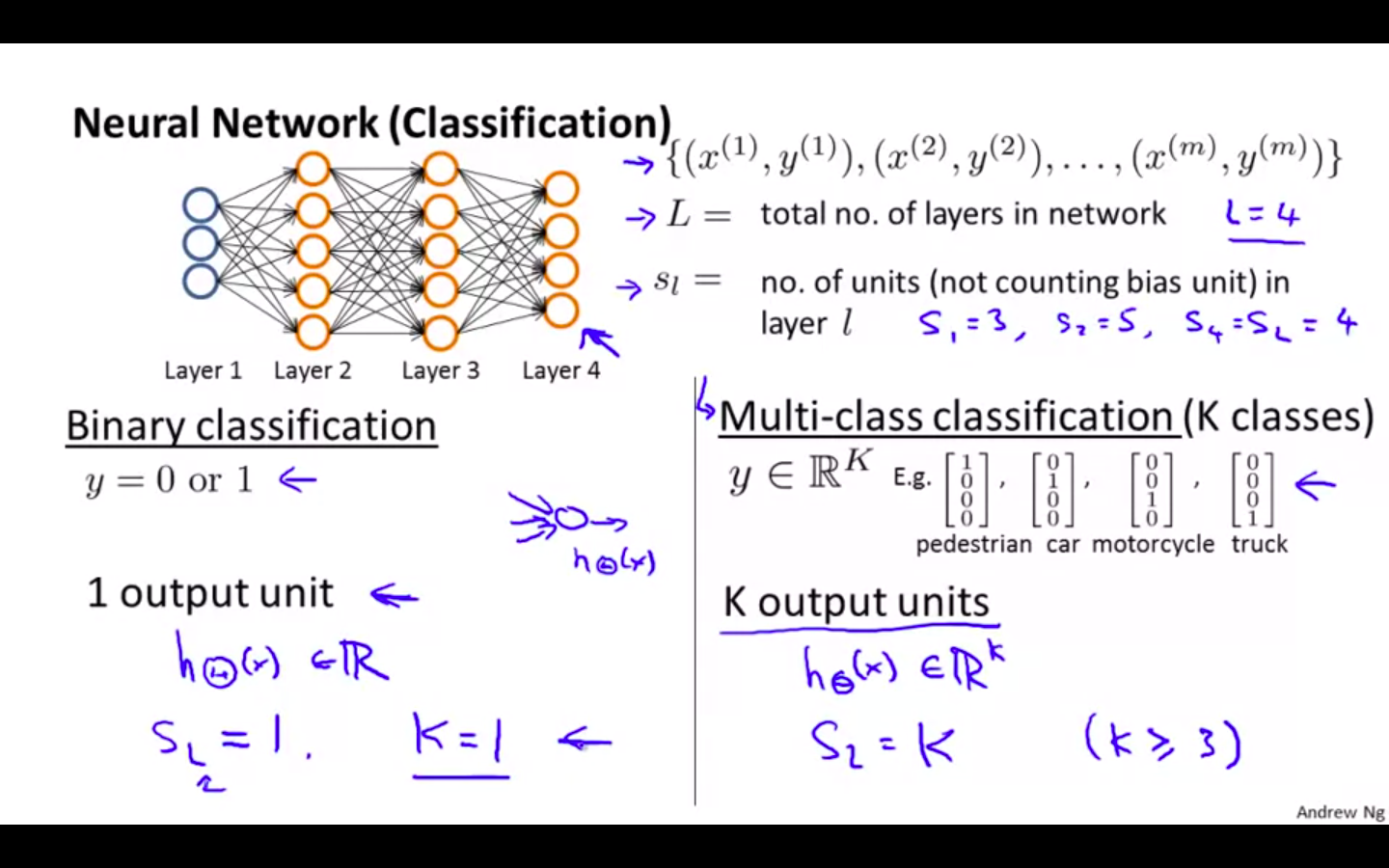
  • L = total number of layers in the network

  • s_l​ = number of units (not counting bias unit) in layer l

  • K = number of output units/classes

• We have added a few nested summations to account for our multiple output nodes.

• In the first part of the equation, before the square brackets, we have an additional nested summation that loops through the number of output nodes.

• In the regularization part, after the square brackets, we must account for multiple theta matrices.

• The number of columns in our current theta matrix is equal to the number of nodes in our current layer (including the bias unit).

• The number of rows in our current theta matrix is equal to the number of nodes in the next layer (excluding the bias unit).

• As before with logistic regression, we square every term.

• Note

  • the double sum simply adds up the logistic regression costs calculated for each cell in the output layer

  • the triple sum simply adds up the squares of all the individual Θs in the entire network.

  • the i in the triple sum does not refer to training example i

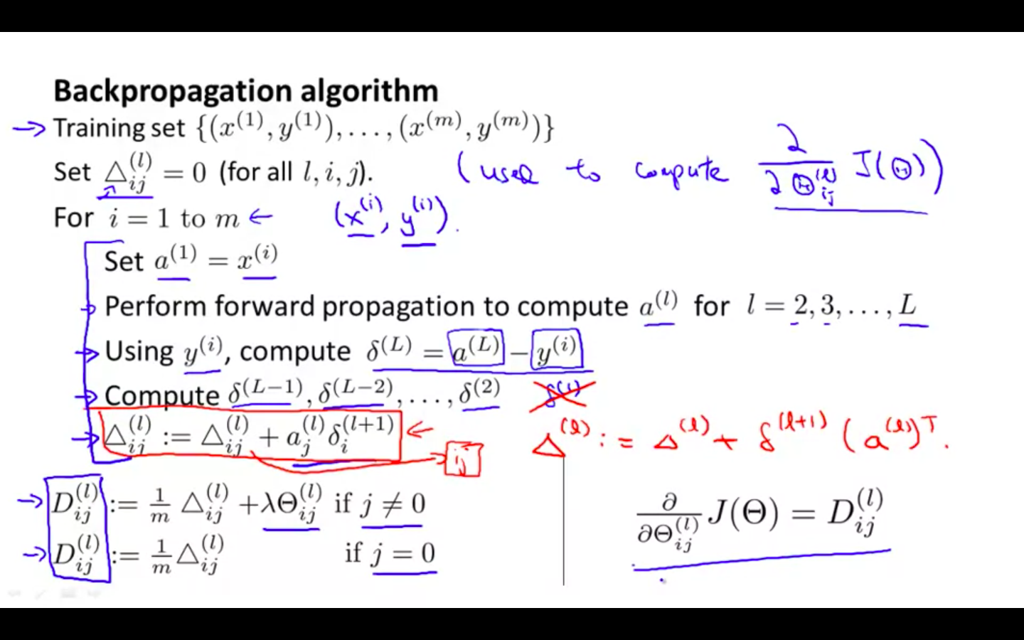
Backpropagation Algorithm

• “Backpropagation” is neural-network terminology for minimizing our cost function, just like what we were doing with gradient descent in logistic and linear regression. Our goal is to compute: min J ( theta )

• That is, we want to minimize our cost function J using an optimal set of parameters in theta.

• To compute the partial derivative of J(Θ):

  • Backpropagation Algorithm is used

• One training example

• Multiple training example

• Process

  

Backpropagation Intuition

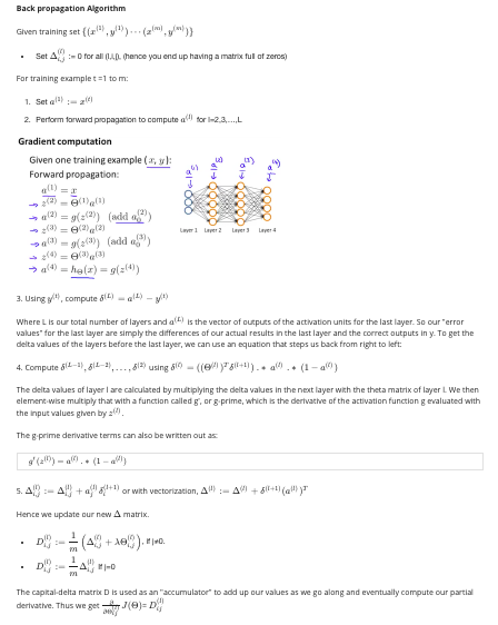
• Forward Propagation

  

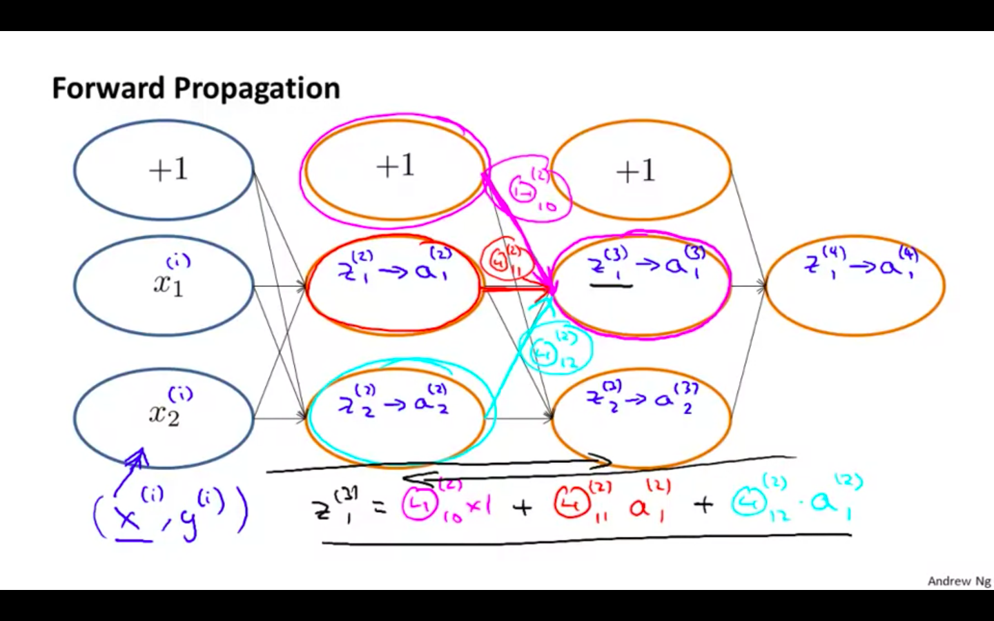
• Backward Propagation

  • The delta values are actually the derivative of the cost function

  • Recall that our derivative is the slope of a line tangent to the cost function, so the steeper the slope the more incorrect we are.

  

Backpropagation in Practice

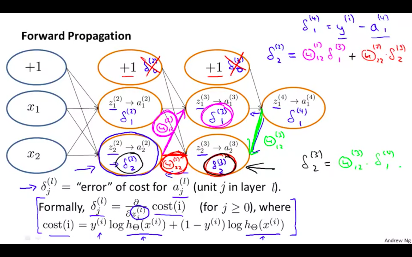
Implementation Note: Unrolling Parameters

• Advance Optimisation

  • It needs theta to be in vectors

  

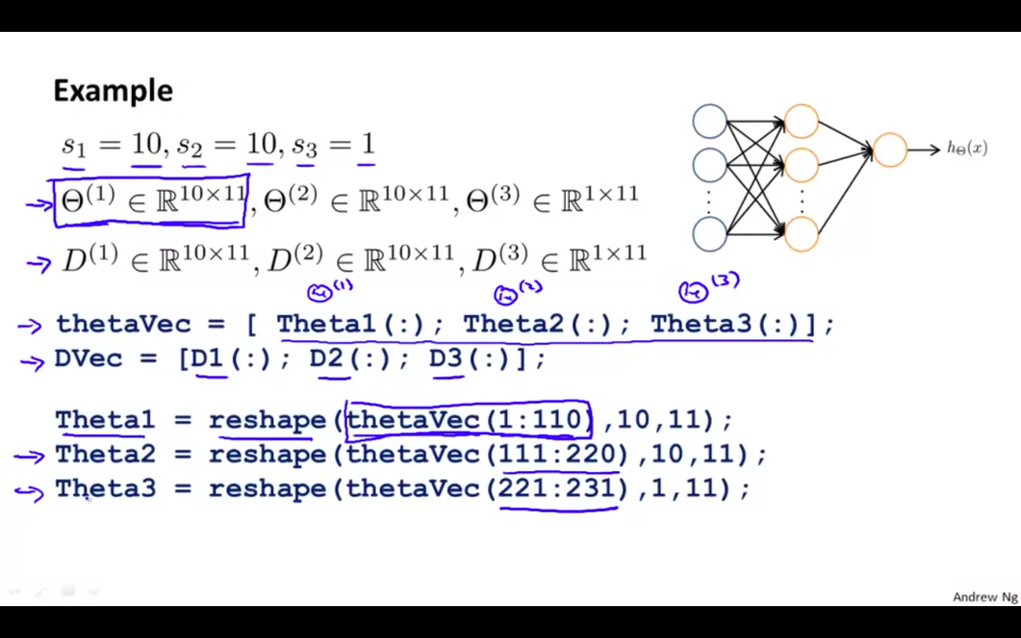
• Example

  • For efficient FP and BP values are expected in matrices and efficient Cost Function are expected in vectors

  • Unrolling matrices into vectors in Octave

  

• Learning Algorithm

  • Process of unrolling

  

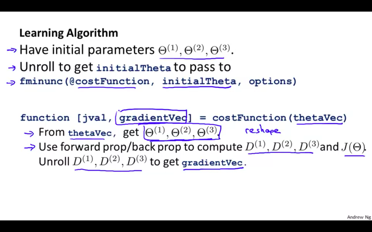
• Octave Snippets

  • Matrices → Vectors

thetaVector = [ Theta1(:); Theta2(:); Theta3(:); ]
deltaVector = [ D1(:); D2(:); D3(:) ]

- Vectors → Matrices

Theta1 = reshape(thetaVector(1:110),10,11)
Theta2 = reshape(thetaVector(111:220),10,11)
Theta3 = reshape(thetaVector(221:231),1,11)

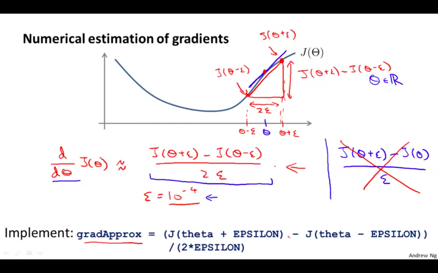
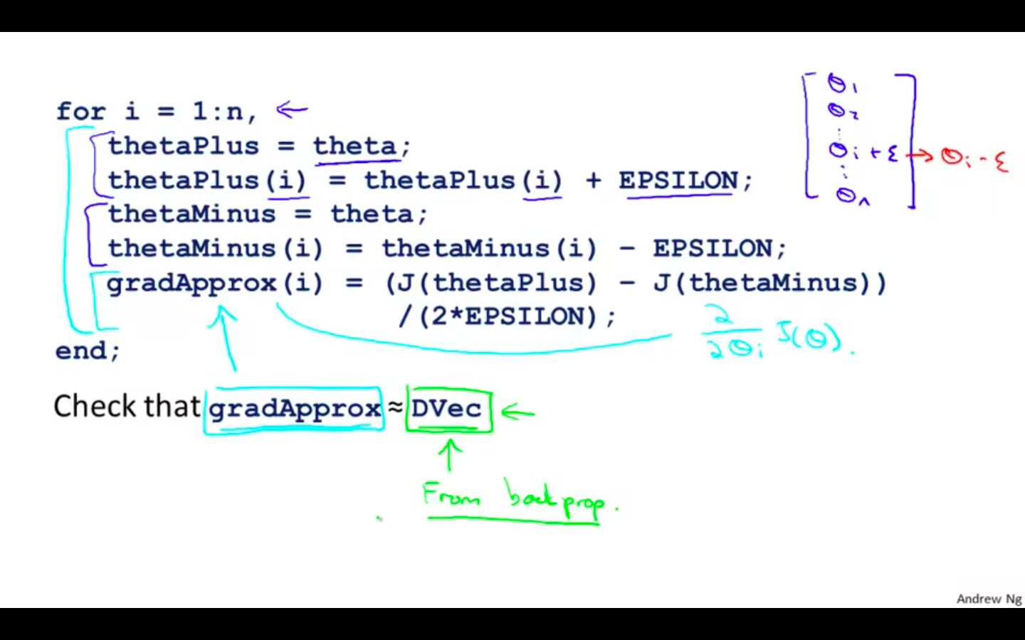
Gradient Checking

• Gradient checking will assure that our backpropagation works as intended.

• We can approximate the derivative of our cost function with:

  • Epsilon = 10^-4 guarantees that the math works out properly.

  • If the value for ϵ\epsilonϵ is too small, we can end up with numerical problems.

  

• Parameter Vector

  

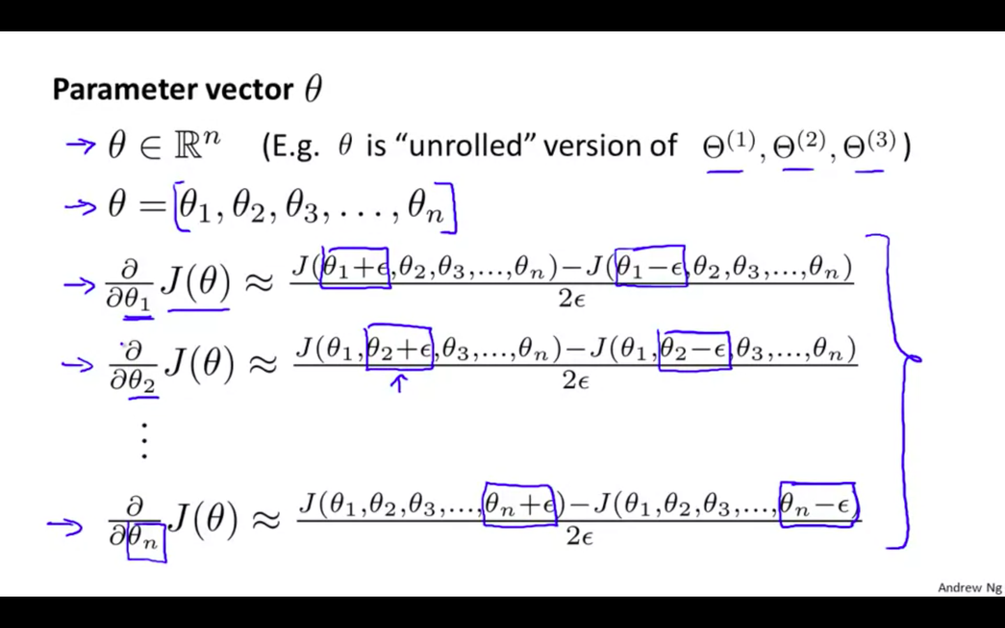
• Process

  • So once we compute our gradApprox vector, we can check that gradApprox ≈ deltaVector.

  

• Notes

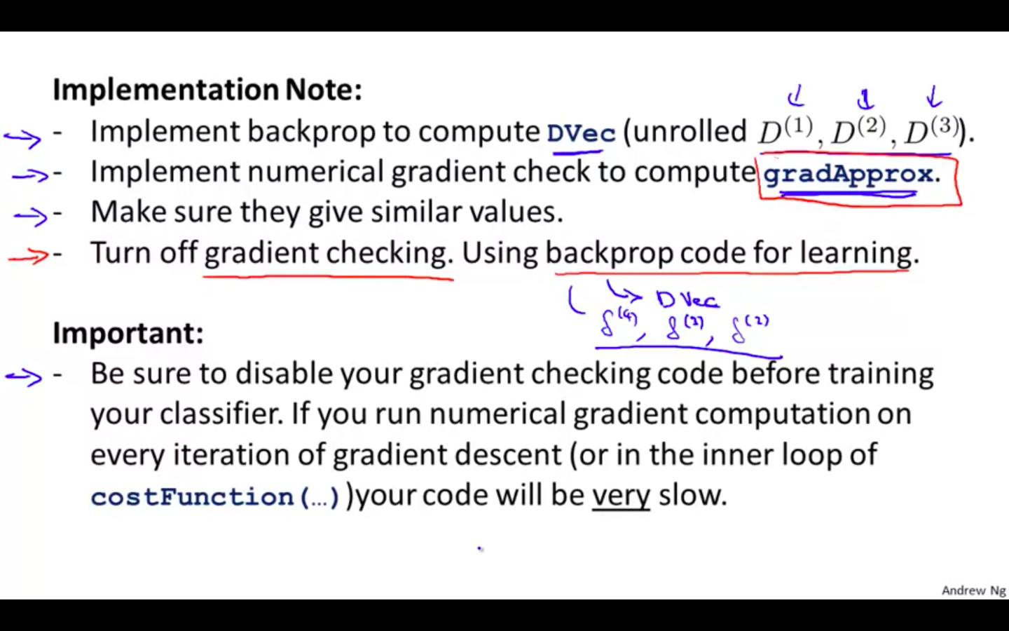
  • Implementation Note

    • Implement BP to compute DVec

    • Implement numerical gradient check to compute gradApprox

    • Make sure they give similar values

    • Turn of gradient checking. Using BP code for learning

  • Important

    • Be sure to disable your gradient checking code before training your classifier.

    • If you run numerical gradient computation on every iteration of gradient descent ( or in the inner loop of costFunction() ) code will be ver slow

  

  • Octave Snippet

epsilon = 1e-4;
for i = 1:n,
  thetaPlus = theta;
  thetaPlus(i) += epsilon;
  thetaMinus = theta;
  thetaMinus(i) -= epsilon;
  gradApprox(i) = (J(thetaPlus) - J(thetaMinus))/(2*epsilon)
end;

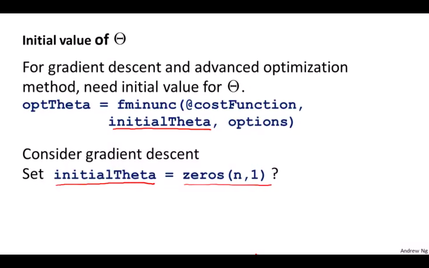
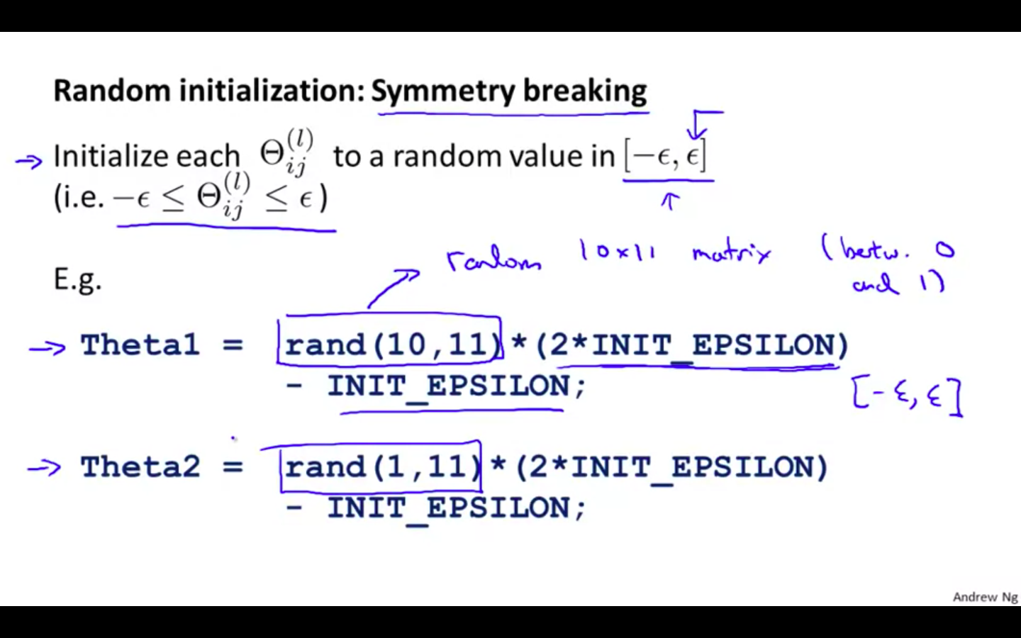
Random Initialisation

• Initial Value of Theta

  • We need the initialise theta

  

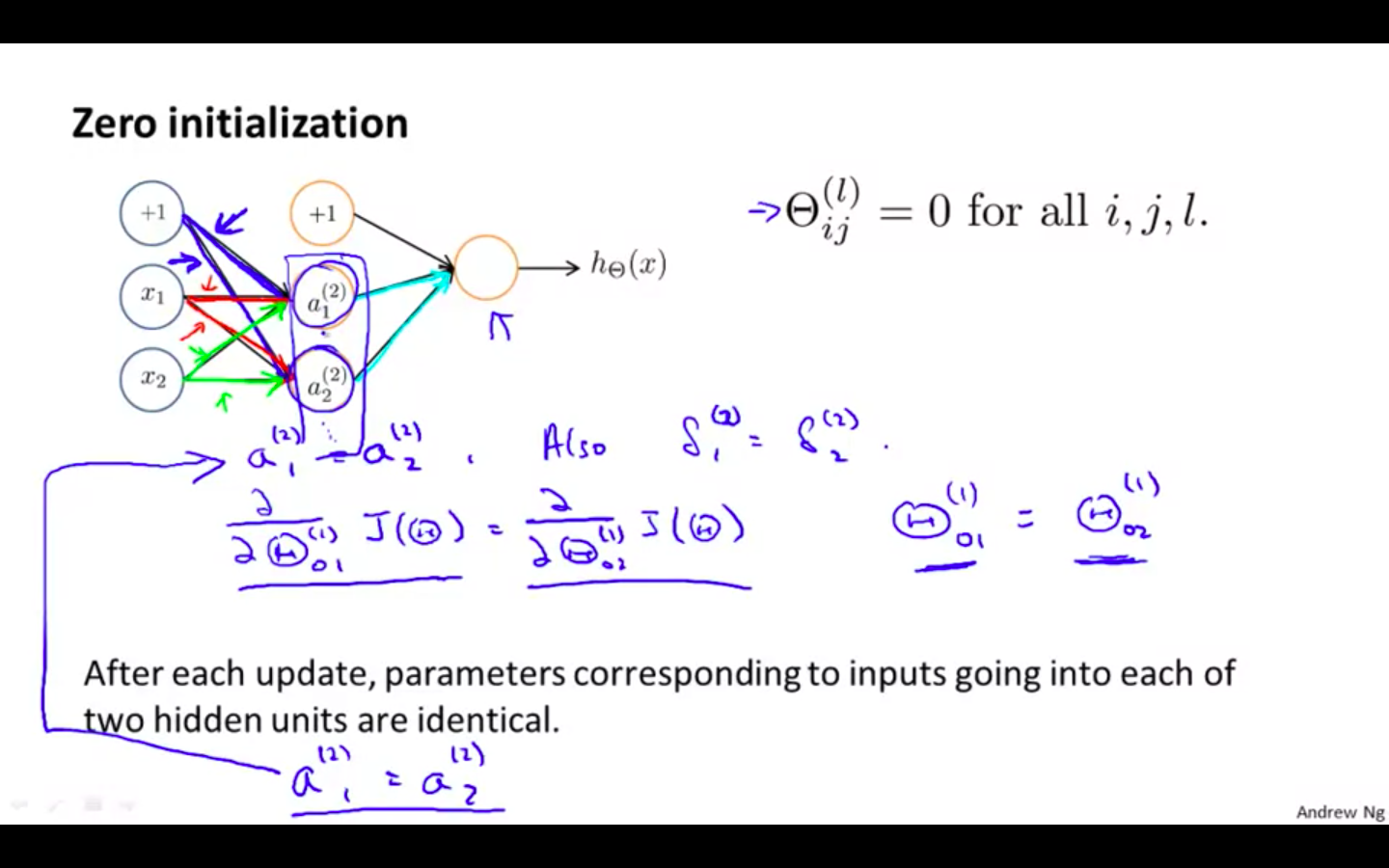
• Zero Initialisation

  • When initialised with zero

  • All the unit in the hidden layer will perform the same activation function

  • Neural Network will not be able to learn for new features

  

• Random Initialisation

  • rand(x,y) is just a function in octave that will initialise a matrix of random real numbers between 0 and 1.

  • (Note: the epsilon used above is unrelated to the epsilon from Gradient Checking)

  

• Octave Snippets

If the dimensions of Theta1 is 10x11, Theta2 is 10x11 and Theta3 is 1x11.

Theta1 = rand(10,11) * (2 * INIT_EPSILON) - INIT_EPSILON;
Theta2 = rand(10,11) * (2 * INIT_EPSILON) - INIT_EPSILON;
Theta3 = rand(1,11) * (2 * INIT_EPSILON) - INIT_EPSILON;

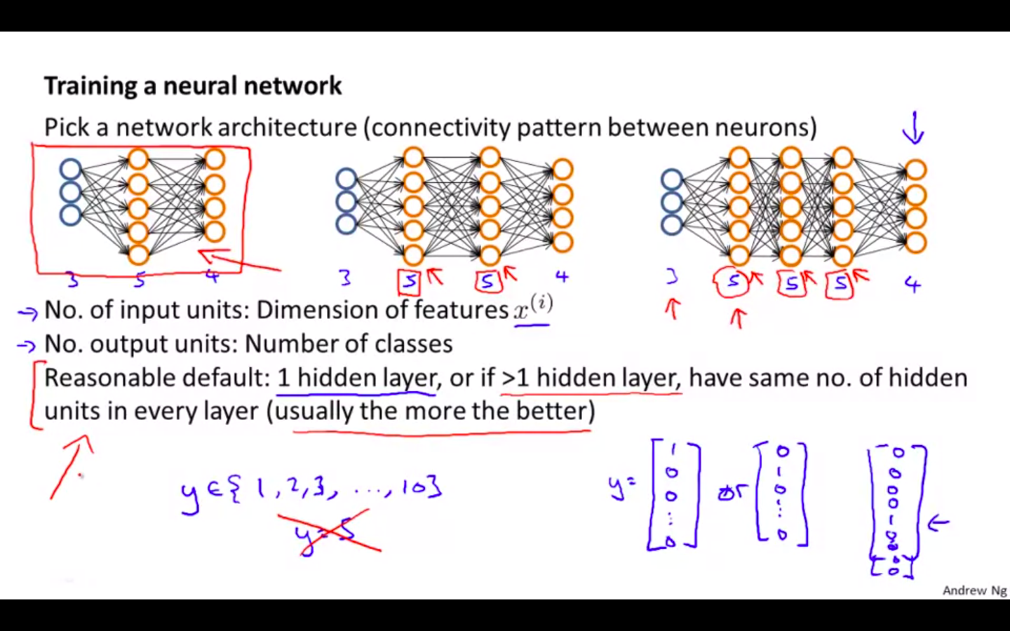
Putting It Together

• First, pick a network architecture; choose the layout of your neural network, including how many hidden units in each layer and how many layers in total you want to have.

  • Number of input units = dimension of features x^i

  • Number of output units = number of classes

  • Number of hidden units per layer = usually more the better (must balance with cost of computation as it increases with more hidden units)

  • Defaults: 1 hidden layer. If you have more than 1 hidden layer, then it is recommended that you have the same number of units in every hidden layer.

  

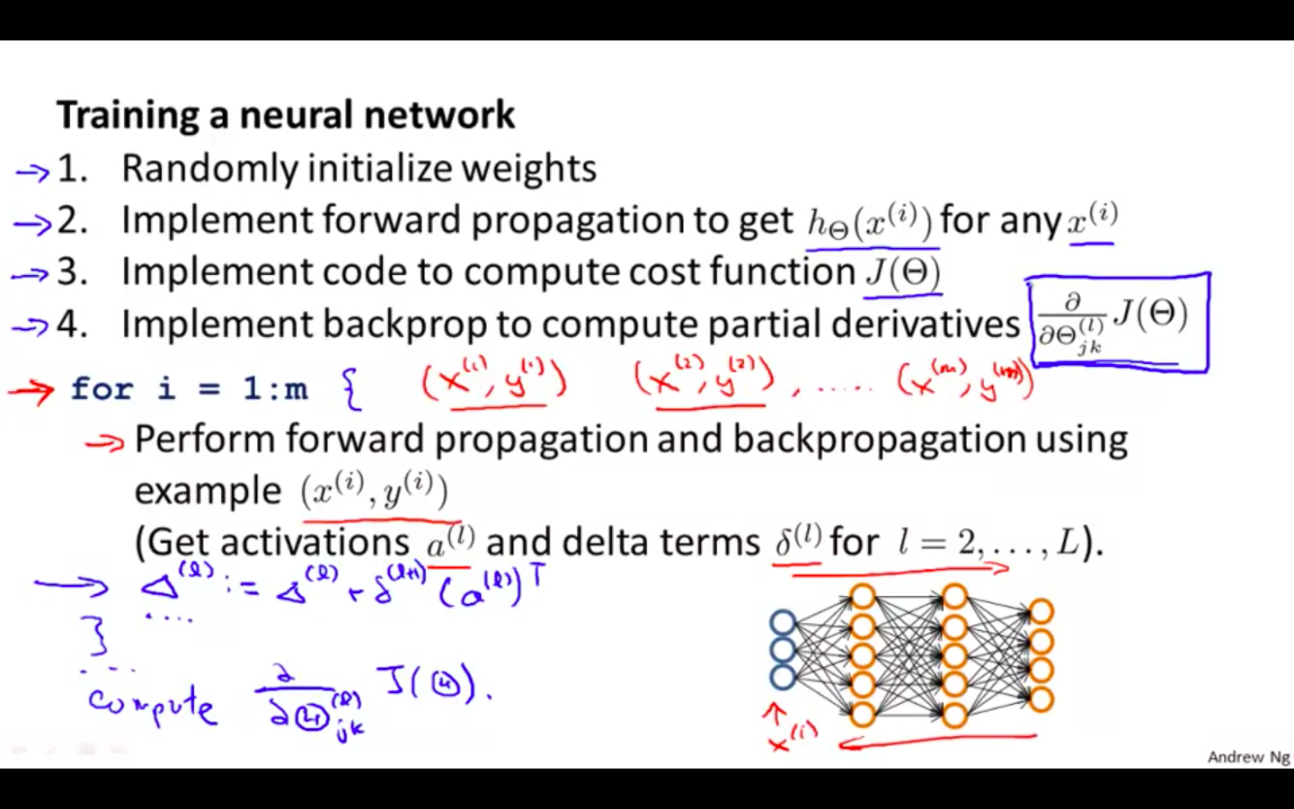
• Training a Neural Network

  1. Randomly initialise the weights

  2. Implement forward propagation to get h(x^i) for any x^i

  3. Implement the cost function

  4. Implement backpropagation to compute partial derivatives

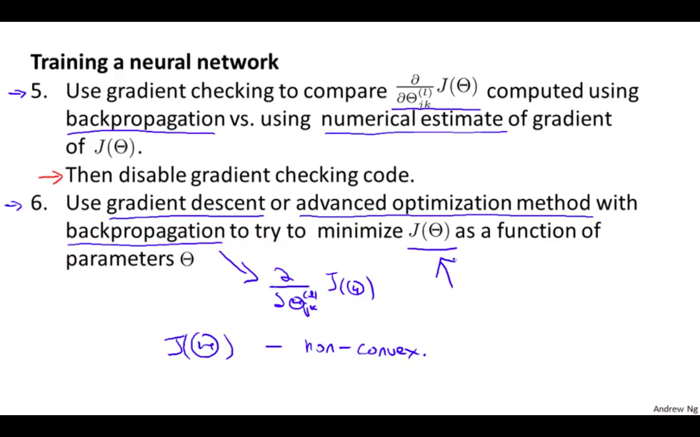
  5. Use gradient checking to confirm that your backpropagation works. Then disable gradient checking.

  6. Use gradient descent or a built-in optimization function to minimize the cost function with the weights in theta.

  • Steps 1 - 4

  

  • Steps 5 - 6

  

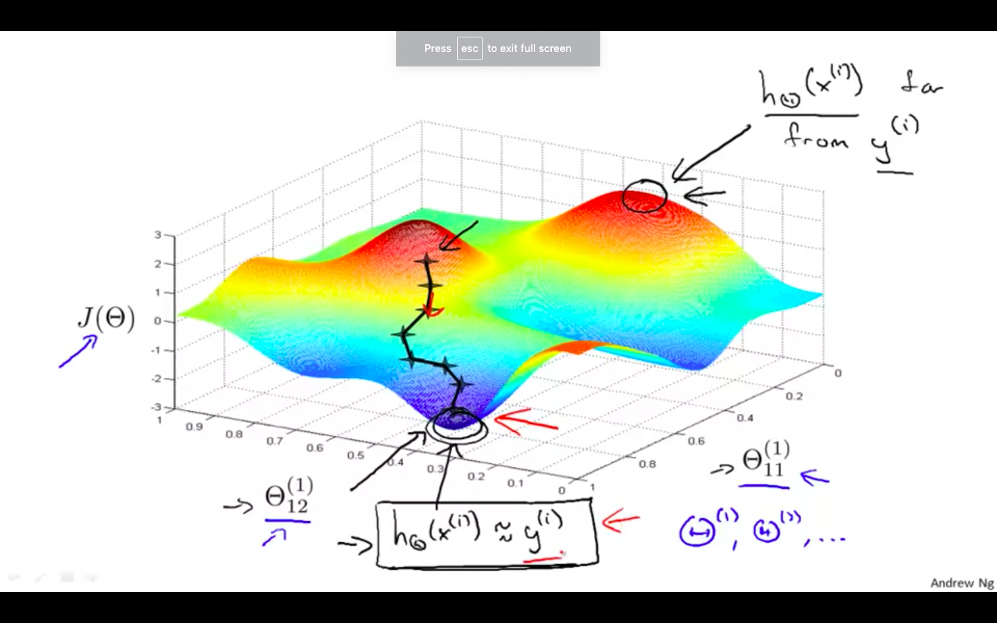
• However, keep in mind that J ( theta ) s not convex and thus we can end up in a local minimum instead.

• Octave Snippets

  • When we perform forward and back propagation, we loop on every training example

for i = 1:m,
   Perform forward propagation and backpropagation using example (x(i),y(i))
   (Get activations a(l) and delta terms d(l) for l = 2,...,L

Application of Neural Networks

Autonomous Driving

Lecture Presentation