Machine Learning By Andew Ng - Week 6
Evaluating a Learning Algorithm
Deciding What to Try Next
-
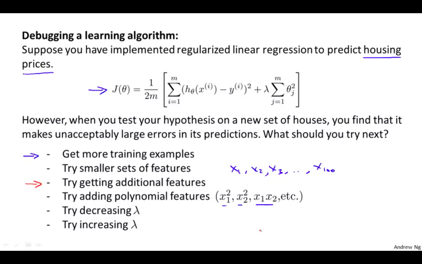
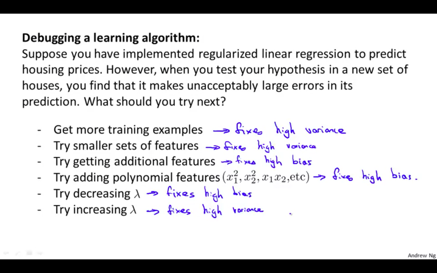
Debugging a learning algorithm
-
What to try next if the hypothesis is making large errors in its predictions
-
Get more training examples
-
Try smaller sets of features
-
Try getting additional features
-
Try decreasing lambda ( regularisation parameter )
-
Try increasing lambda ( regularisation parameter )
-
-
-
Diagnostics
-
A test that you can run to gain insight what is / isn’t working with a learning algorithm, and gain guidance as to how best to improve its performance.
-
Diagnostics can take time to implement, but doing so can be a very good use of your time.
-
Evaluating a Hypothesis
-
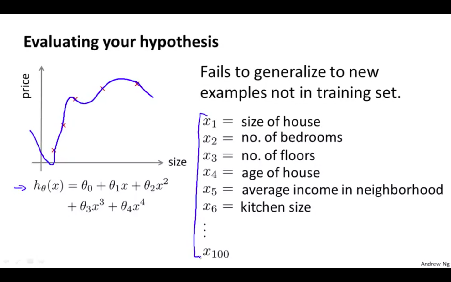
A hypothesis may have a low error for the training examples but still be inaccurate (because of overfitting).
-
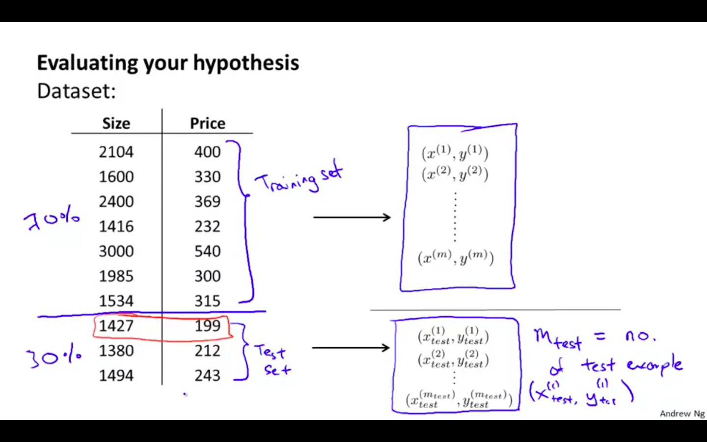
Thus, to evaluate a hypothesis, given a dataset of training examples, we can split up the data into two sets: a training set and a test set.
-
Typically, the training set consists of 70 % of your data and the test set is the remaining 30 %.
-
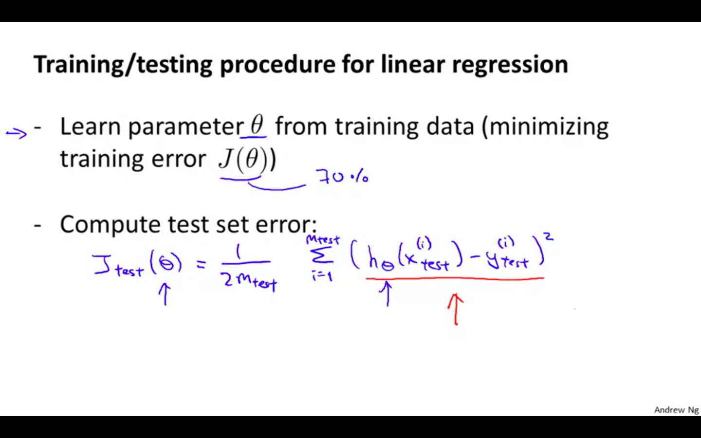
The new procedure using these two sets is then:
-
Learn Θ and minimise J_train(Θ) using the training set
-
Compute the test set error J_test(Θ)
-
-
Linear Regression
-
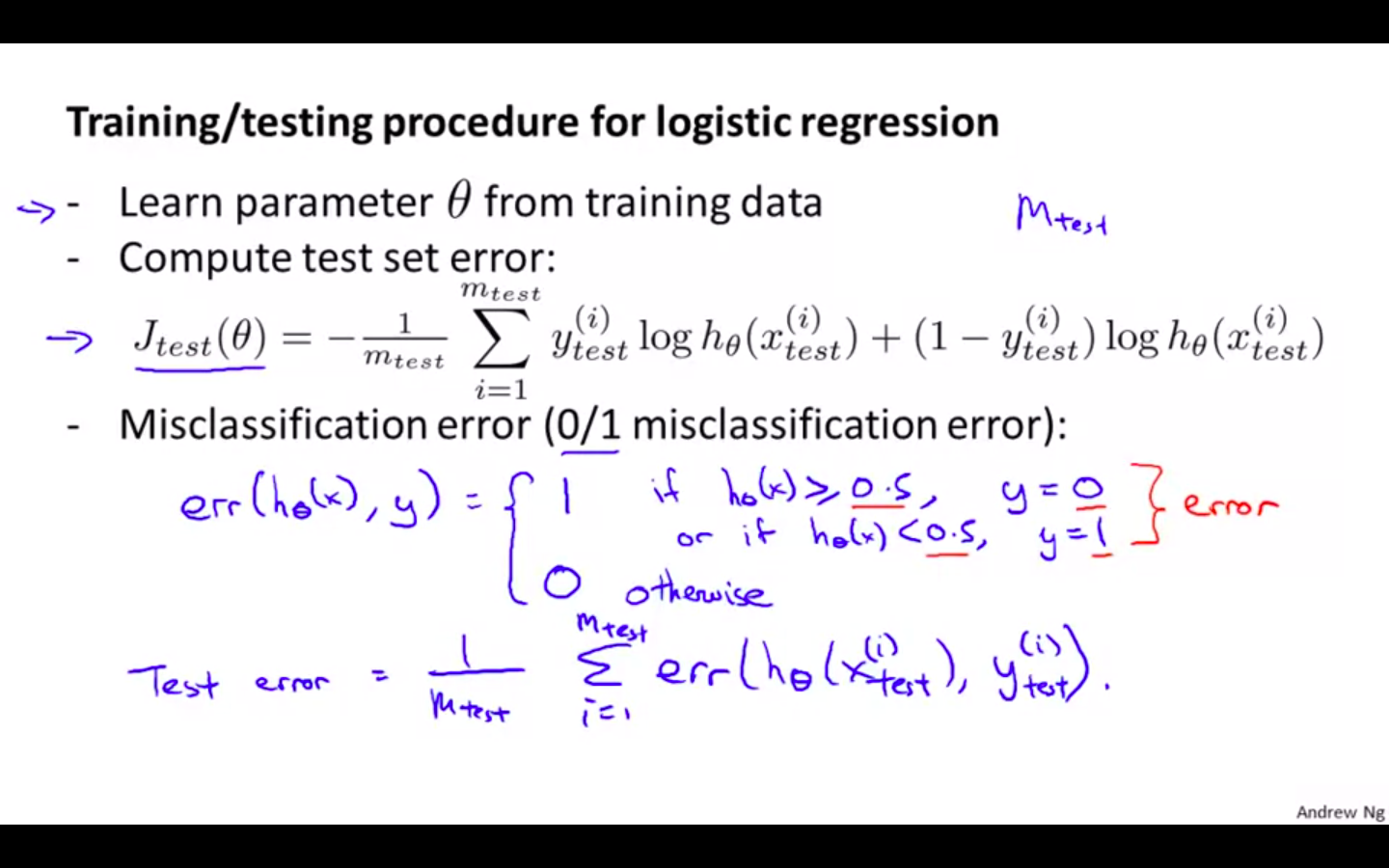
Logistic Regression
-
For classification ~ Misclassification error (aka 0/1 misclassification error)
-
This gives us a binary 0 or 1 error result based on a misclassification. The average test error for the test set is
-
This gives us the proportion of the test data that was misclassified.
-
-
Model Selection and Train/Validation/Test Sets
-
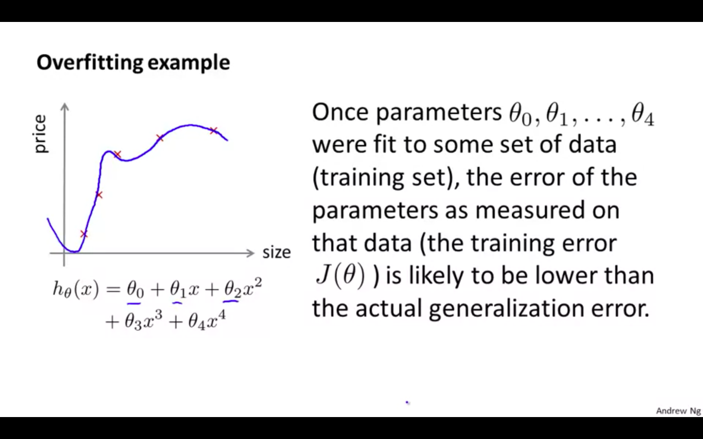
Just because a learning algorithm fits a training set well, that does not mean it is a good hypothesis.
-
It could over fit and as a result your predictions on the test set would be poor.
-
The error of your hypothesis as measured on the data set with which you trained the parameters will be lower than the error on any other data set.
-
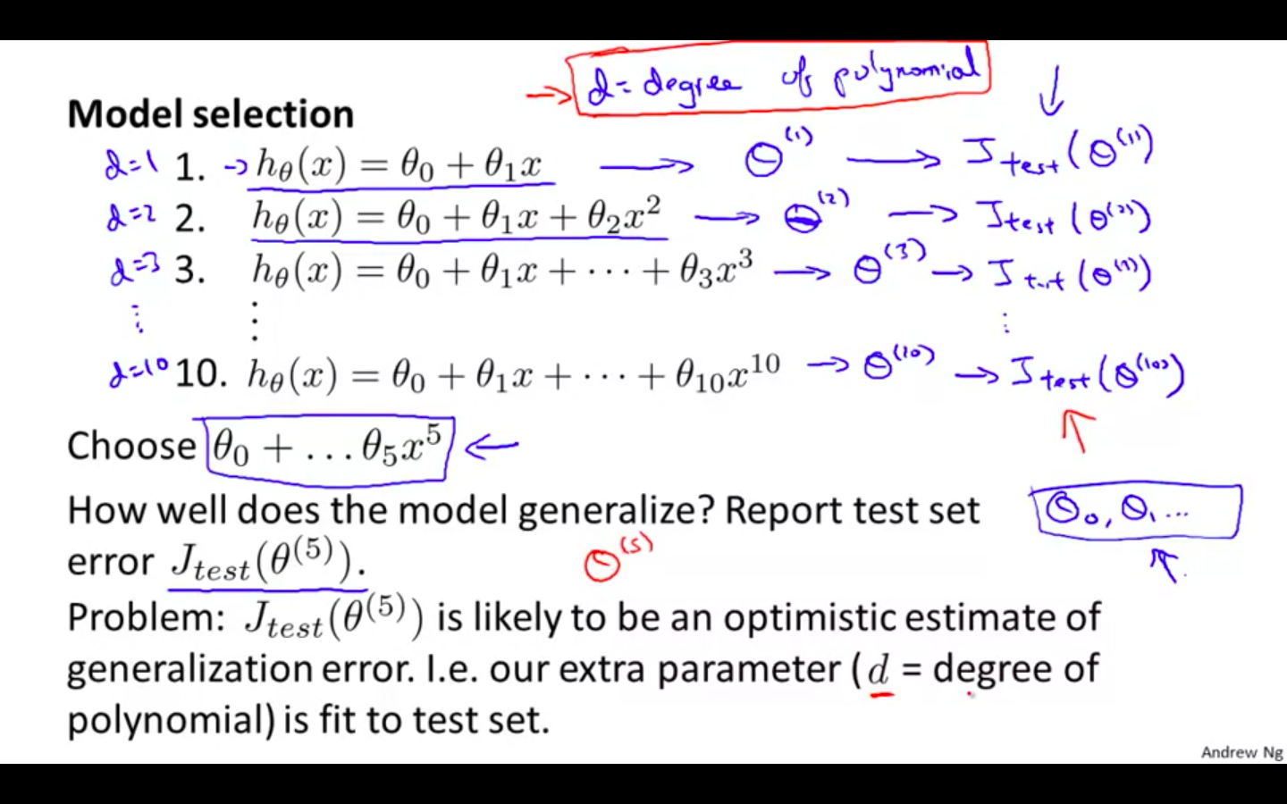
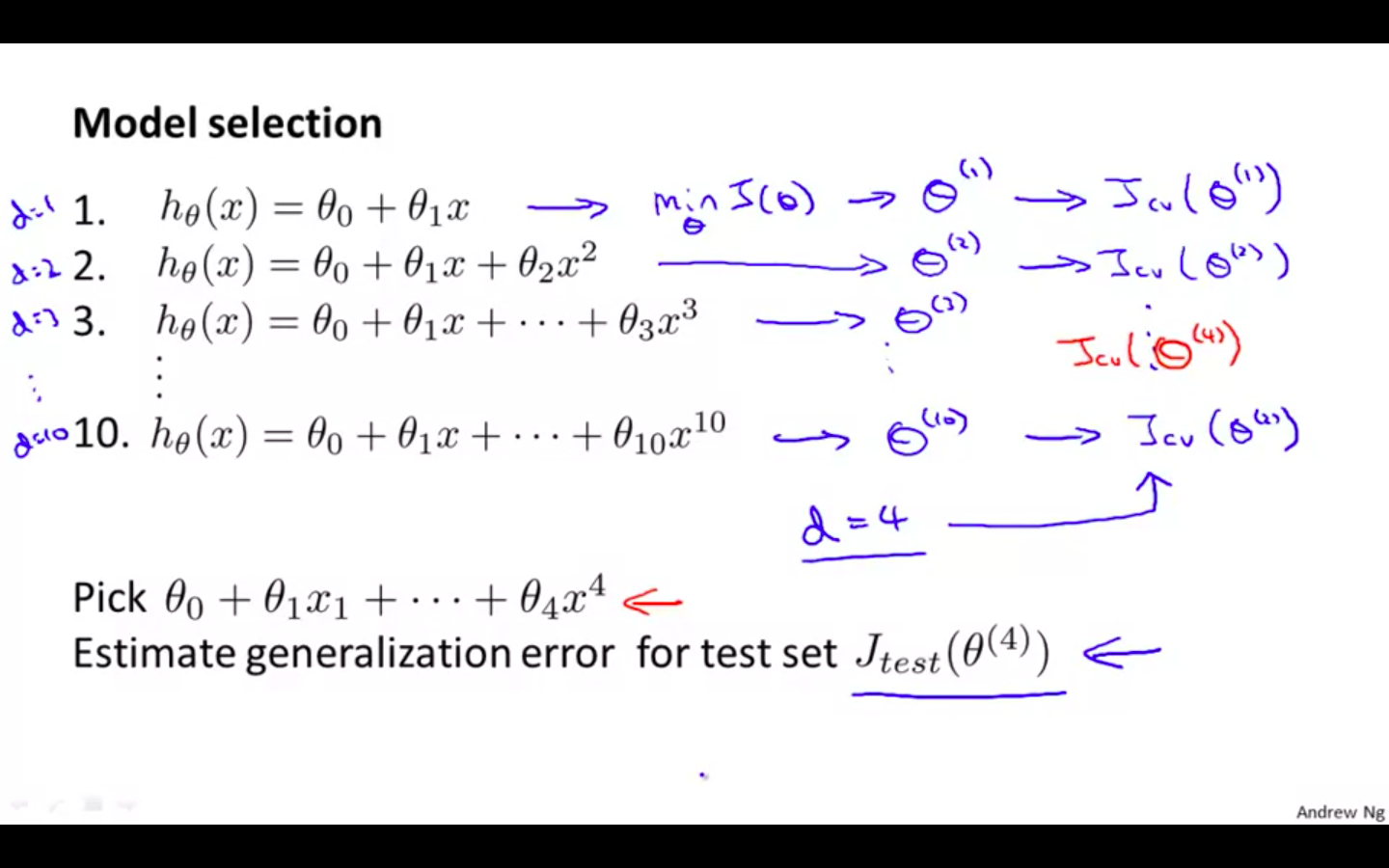
Given many models with different polynomial degrees, we can use a systematic approach to identify the ‘best’ function.
-
In order to choose the model of your hypothesis, you can test each degree of polynomial and look at the error result.
-
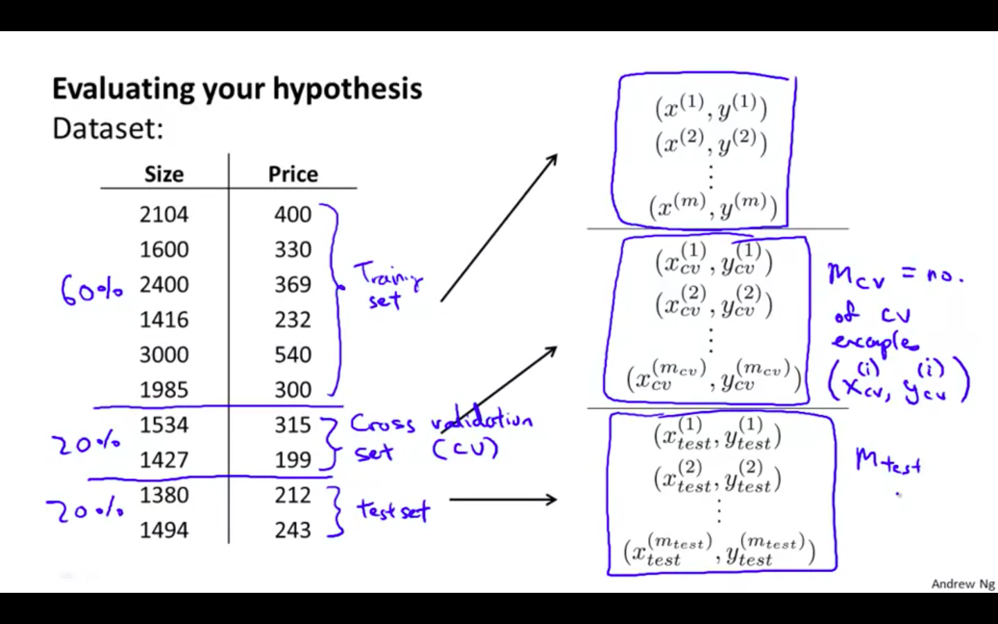
One way to break down our dataset into the three sets is:
-
Training set: 60%
-
Cross validation set: 20%
-
Test set: 20%
-
-
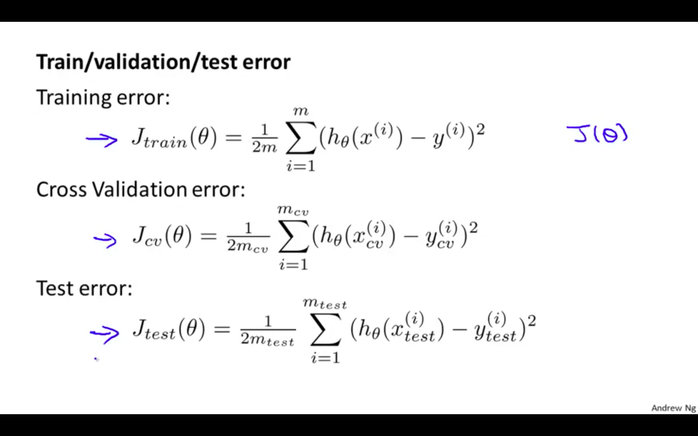
We can now calculate three separate error values for the three different sets using the following method:
-
Optimise the parameters in Θ using the training set for each polynomial degree.
-
Find the polynomial degree d with the least error using the cross validation set.
-
Estimate the generalisation error using the test set with J_test(Θ^(d)), (d = theta from polynomial with lower error);
-
This way, the degree of the polynomial d has not been trained using the test set.
-
Bias vs Variance
Diagnosing Bias vs Variance
-
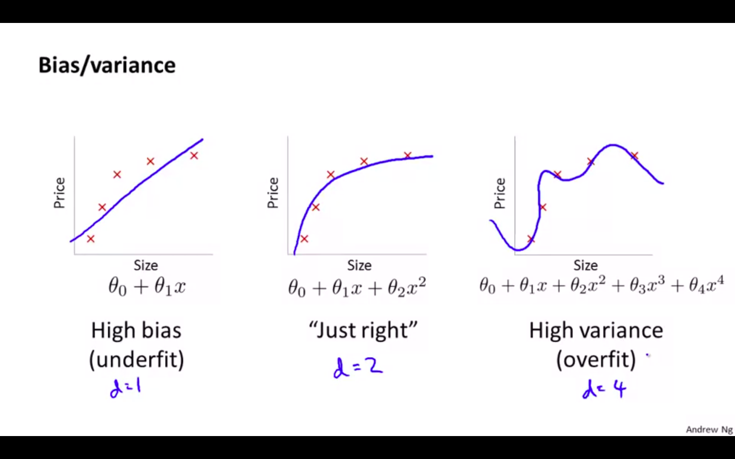
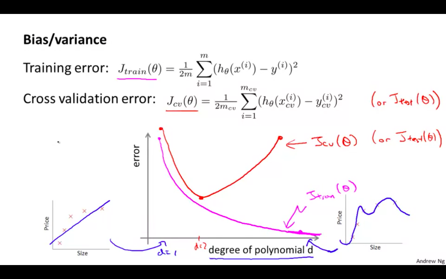
The relationship between the degree of the polynomial d and the underfitting or overfitting of our hypothesis.
-
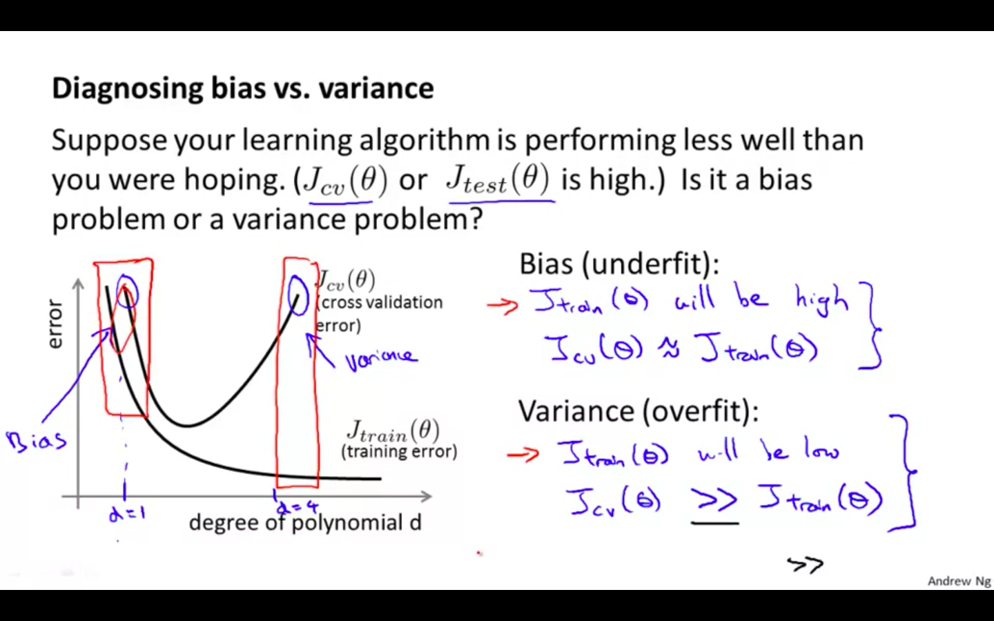
We need to distinguish whether bias or variance is the problem contributing to bad predictions.
-
High bias is underfitting and high variance is overfitting. Ideally, we need to find a golden mean between these two.
-
The training error will tend to decrease as we increase the degree d of the polynomial.
-
At the same time, the cross validation error will tend to decrease as we increase d up to a point, and then it will increase as d is increased, forming a convex curve.
-
High bias (underfitting): both J_train(theta) and J_cv(thetha) will be high
-
High variance (overfitting): J_train(theta) will be low and J_cv(thetha) will be much greater than the other
-
Regularisation and Bias / Variance
-
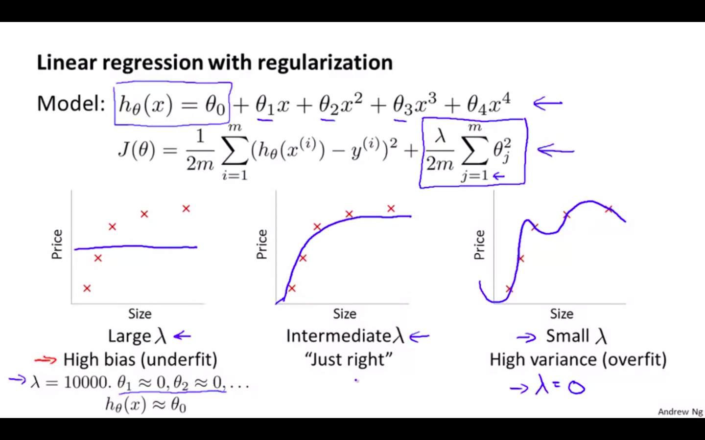
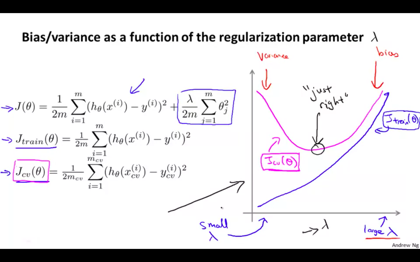
As λ increases, our fit becomes more rigid. On the other hand, as λ approaches 0, we tend to over overfit the data.
-
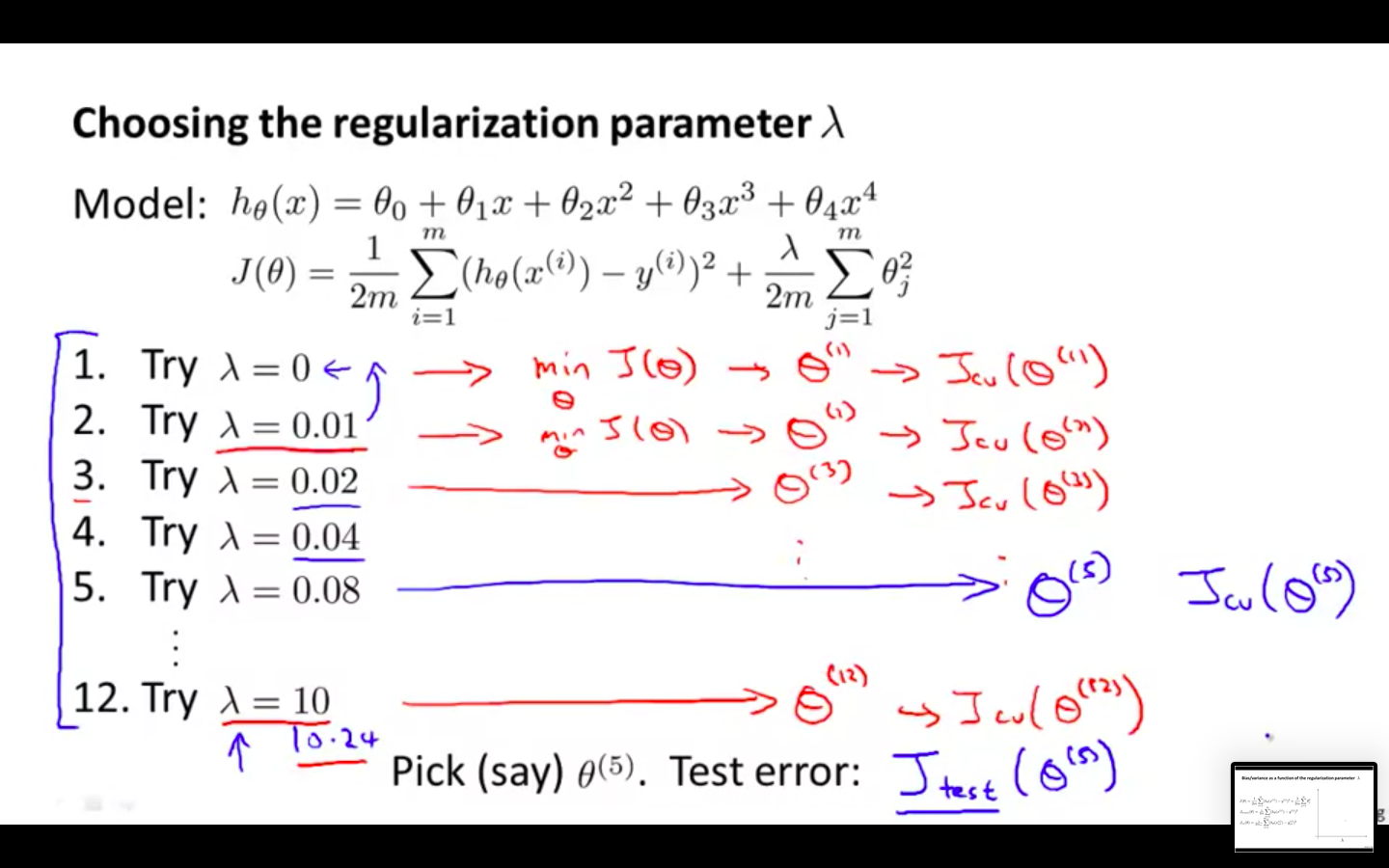
How do we choose our parameter λ to get it ‘just right’ ? In order to choose the model and the regularisation term λ
-
We need to:
-
Create a list of lambdas (i.e. λ∈{0,0.01,0.02,0.04,0.08,0.16,0.32,0.64,1.28,2.56,5.12,10.24});
-
Create a set of models with different degrees or any other variants.
-
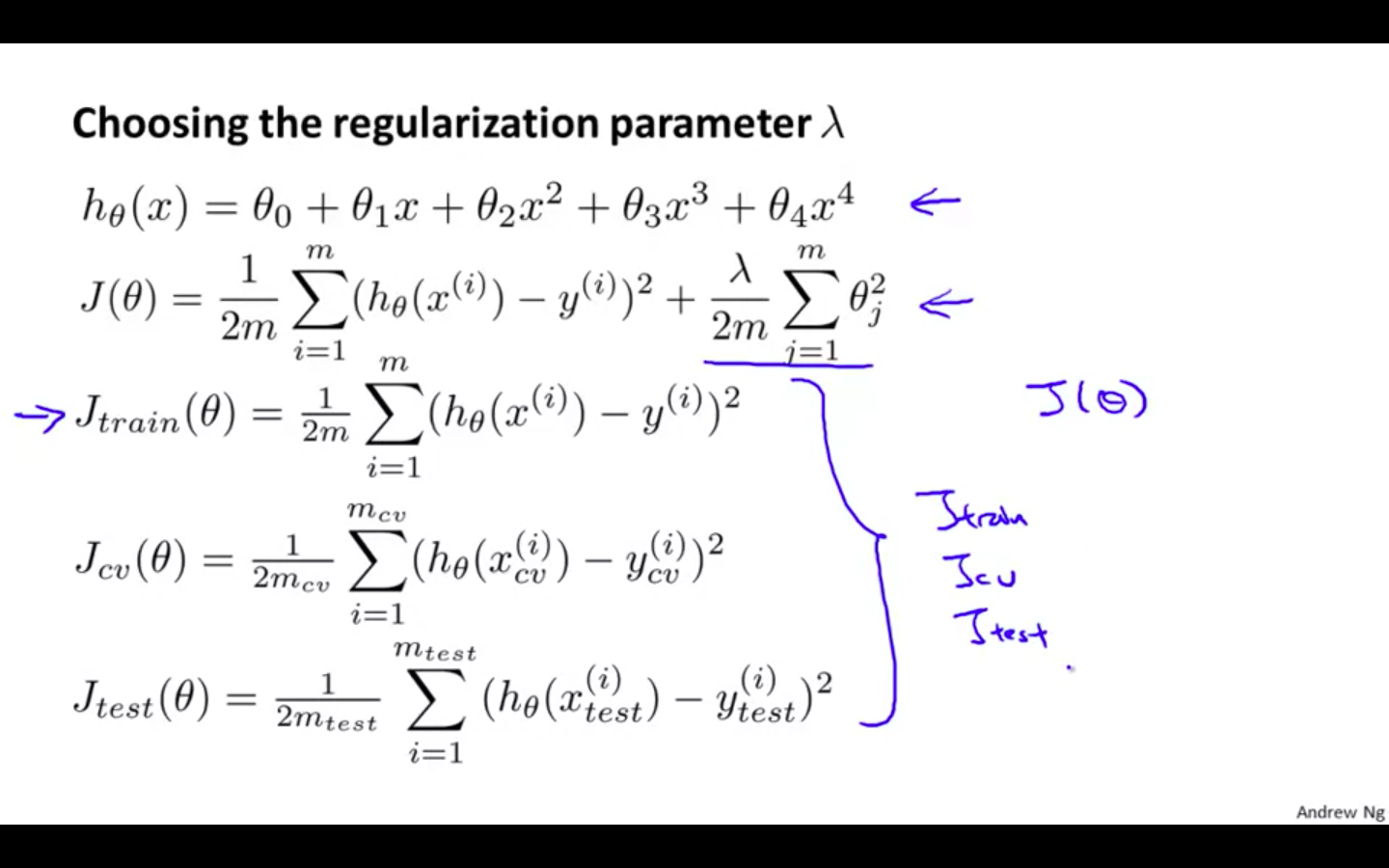
Iterate through the λs and for each λ go through all the models to learn some Θ.
-
Compute the cross validation error using the learned Θ (computed with λ) on the J_CV(Θ) **without **regularisation or λ = 0.
-
Select the best combo that produces the lowest error on the cross validation set.
-
Using the best combo Θ and λ, apply it on J_test(Θ) to see if it has a good generalisation of the problem.
-
-
-
Bias / Variance against Regularisation Parameter
Learning Curves
-
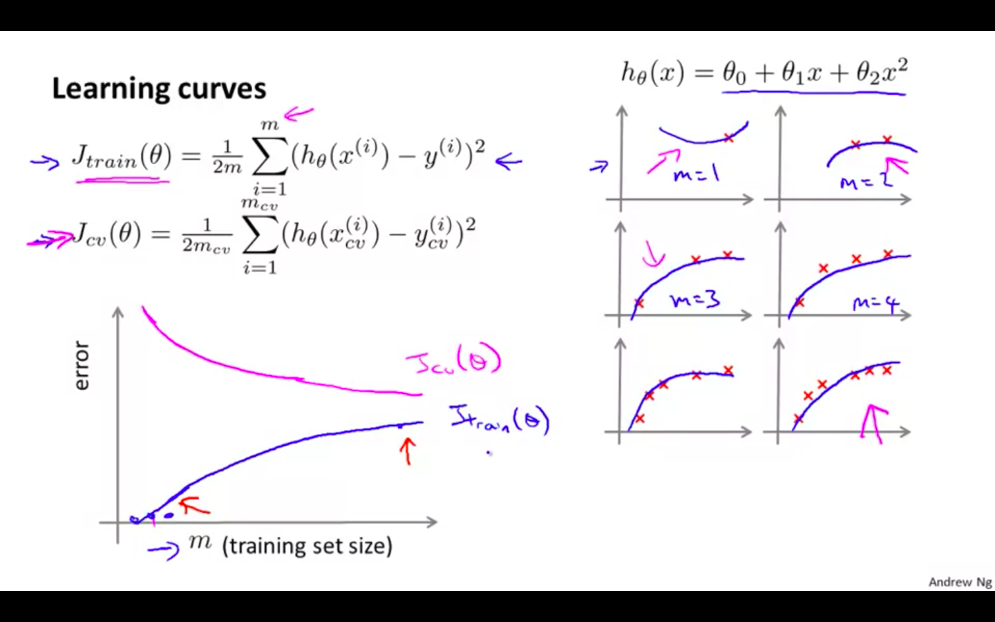
Training an algorithm on a very few number of data points (such as 1, 2 or 3) will easily have 0 errors because we can always find a quadratic curve that touches exactly those number of points.
-
Hence
-
As the training set gets larger, the error for a quadratic function increases.
-
The error value will plateau out after a certain m, or training set size.
-
-
Learning Curves when there is High Bias
-
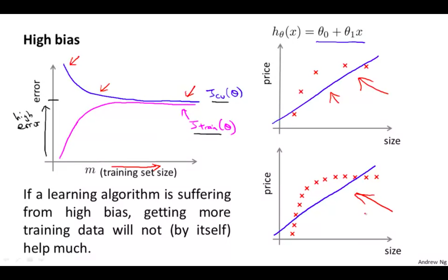
Low training set size : J_train(theta) to be low and J_cv(theta) to be high
-
Large training set size: J_train(theta) and J_cv(theta) to be high with both similar
-
If a learning algorithm is suffering from high bias, getting more training data will not (by itself) help much.
-
-
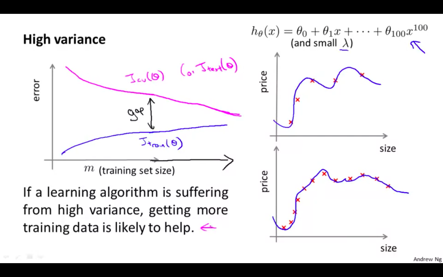
Learning Curves where is High Variance
-
Low training set size : J_train(theta) to be low and J_cv(theta) to be high
-
Large training set size: J_train(theta) increases with training set size and J_cv(theta) continues to decrease without levelling off. Also train < cv but the difference between them remains significant
-
If a learning algorithm is suffering from high variance, getting more training data is likely to help
-
Deciding What To Do Next Revisited
-
Our decision process can be broken down as follows
-
Getting more training examples: Fixes high variance
-
Trying smaller sets of features: Fixes high variance
-
Adding features: Fixes high bias
-
Adding polynomial features: Fixes high bias
-
Decreasing λ: Fixes high bias
-
Increasing λ: Fixes high variance.
-
-
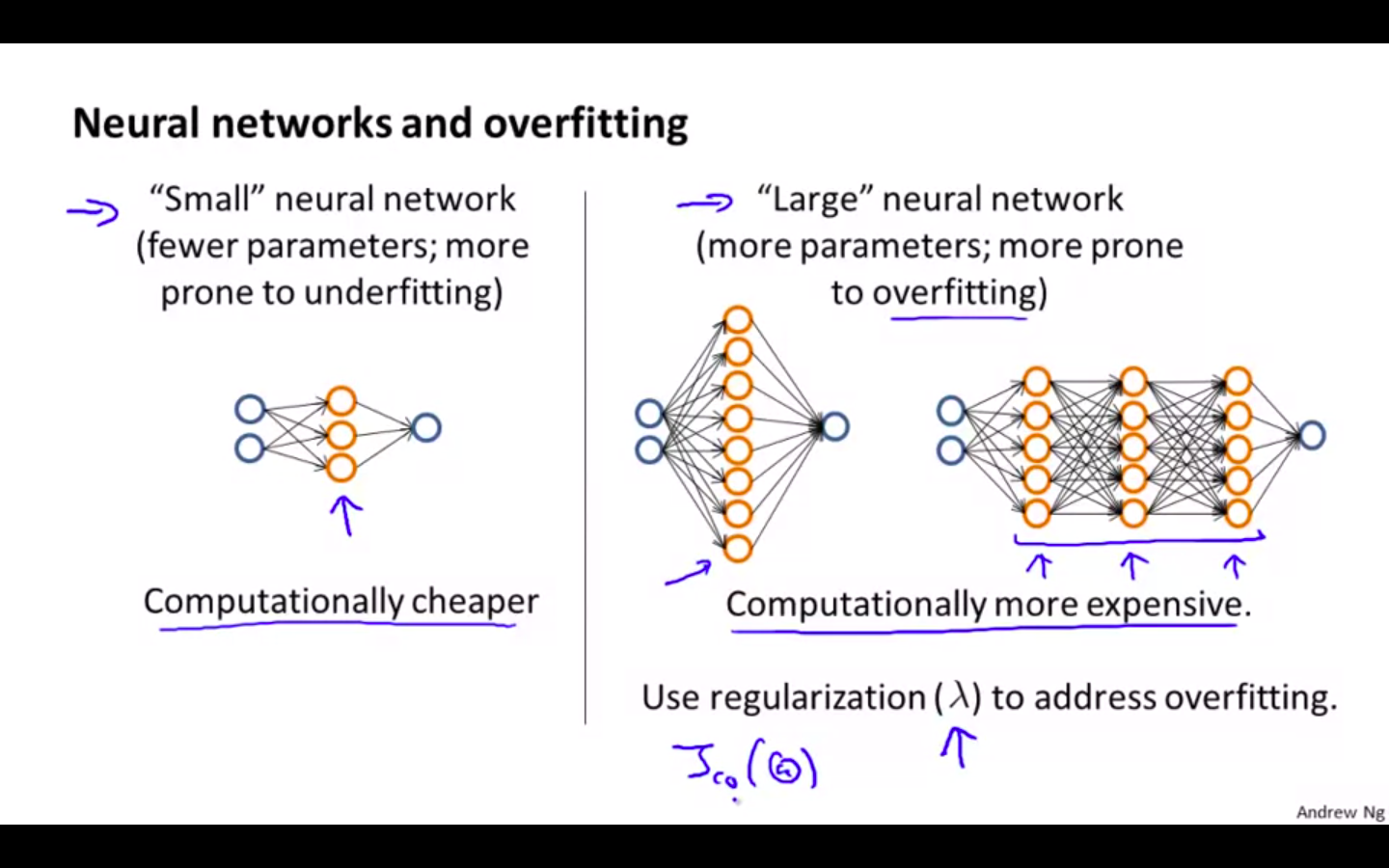
Diagnosing Neural Network
-
A neural network with fewer parameters is prone to underfitting. It is also computationally cheaper.
-
A large neural network with more parameters is prone to overfitting.
-
It is also computationally expensive. In this case you can use regularisation (increase λ) to address the overfitting.
-
Using a single hidden layer is a good starting default. You can train your neural network on a number of hidden layers using your cross validation set. You can then select the one that performs best.
-
-
Model Complexity Effects
-
Lower-order polynomials (low model complexity) have high bias and low variance. In this case, the model fits poorly consistently.
-
Higher-order polynomials (high model complexity) fit the training data extremely well and the test data extremely poorly. These have low bias on the training data, but very high variance.
-
In reality, we would want to choose a model somewhere in between, that can generalise well but also fits the data reasonably well.
-
Building a Spam Classifier
Prioritising What to Work On
-
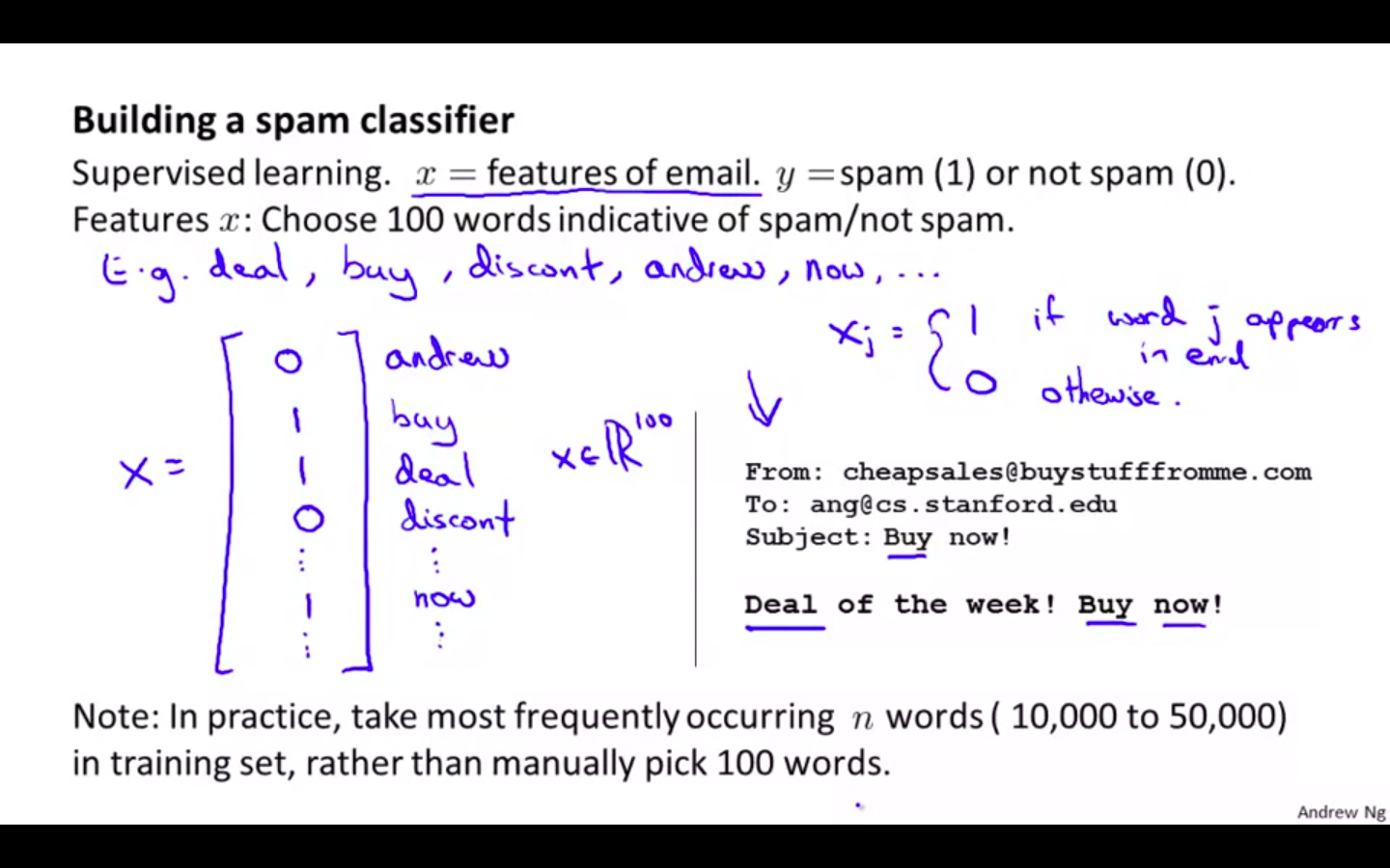
Spam Classifier

-
System Design Example
-
Given a data set of emails, we could construct a vector for each email. Each entry in this vector represents a word.
-
The vector normally contains 10,000 to 50,000 entries gathered by finding the most frequently used words in our data set.
-
If a word is to be found in the email, we would assign its respective entry a 1, else if it is not found, that entry would be a 0.
-
Once we have all our x vectors ready, we train our algorithm and finally, we could use it to classify if an email is a spam or not.
-
-
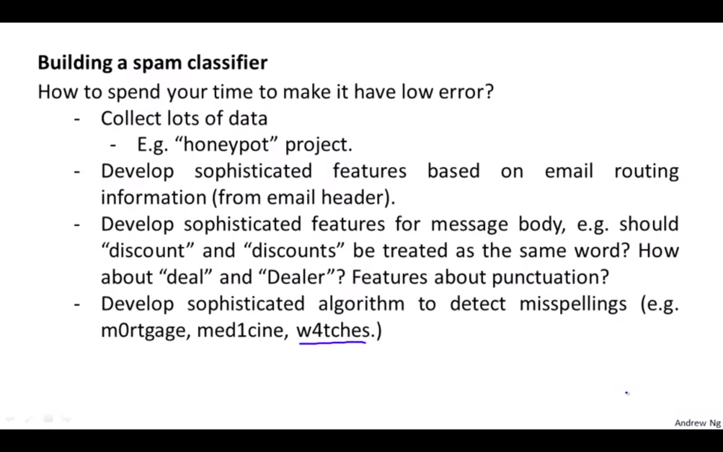
What to prioritise on ? Spend more time on ?
-
Collect lots of data
- E.g. “honeypot” project
-
Develop sophisticated features based on email routing information ( from email header )
-
Develop sophisticated features for message body, e.g. should “discount” and “discounts” be treated as the same word? How about “deal” and “Dealer”? Features about punctuation?
-
Develop sophisticated algorithm to detect misspellings ( e.g. m0rtgage, med1cine, w4tches )
-
It is difficult to tell which of the options will be most helpful.
-
Error Analysis
-
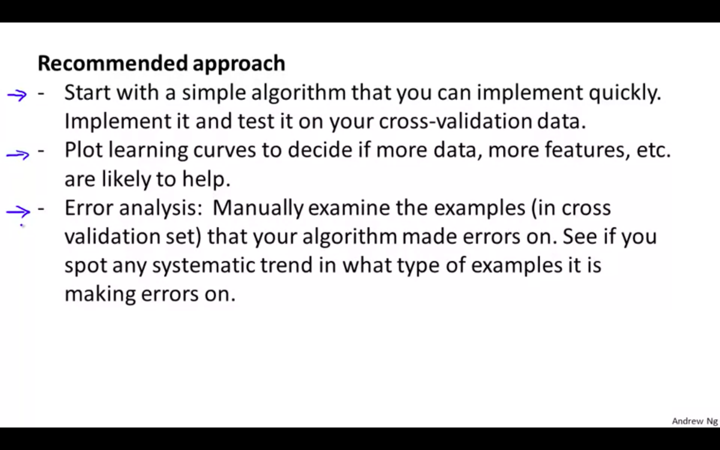
The recommended approach to solving machine learning problems is to
-
Start with a simple algorithm, implement it quickly, and test it early on your cross validation data.
-
Plot learning curves to decide if more data, more features, etc. are likely to help.
-
Manually examine the errors on examples in the cross validation set and try to spot a trend where most of the errors were made.
-
-
Error Analysis
-
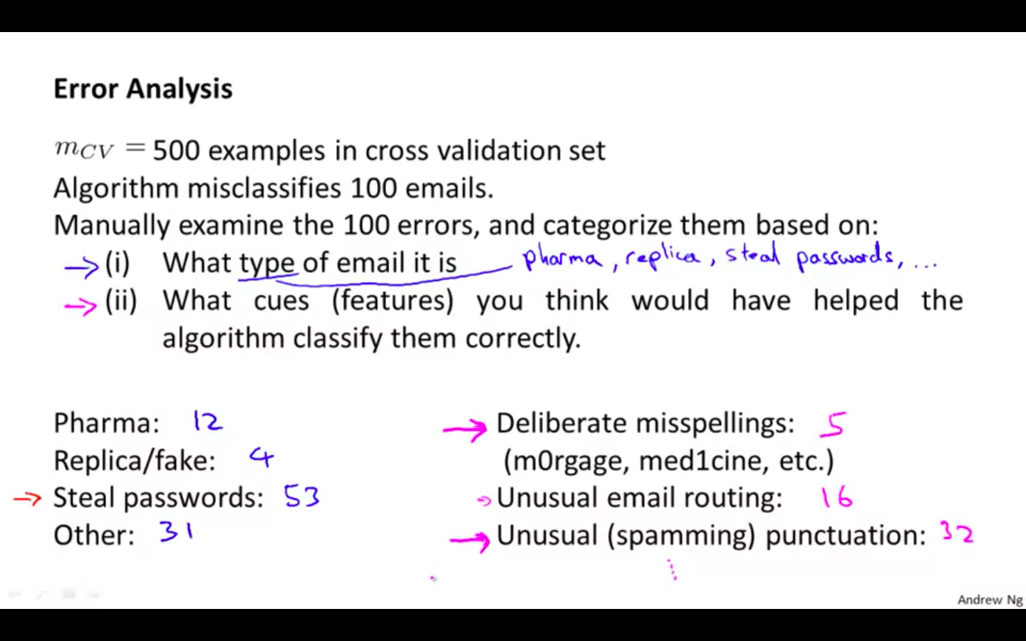
For example, assume that we have 500 emails and our algorithm misclassifies a 100 of them.
-
We could manually analyse the 100 emails and categorise them based on what type of emails they are. We could then try to come up with new cues and features that would help us classify these 100 emails correctly.
-
Hence, if most of our misclassified emails are those which try to steal passwords, then we could find some features that are particular to those emails and add them to our model.
-
We could also see how classifying each word according to its root changes our error rate.
-
-
Importance of Numerical Evaluation
-
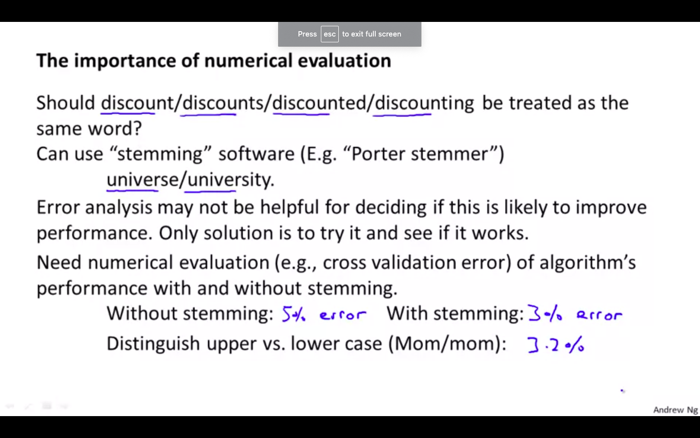
It is very important to get error results as a single, numerical value. Otherwise it is difficult to assess your algorithm’s performance.
-
For example if we use stemming, which is the process of treating the same word with different forms (fail/failing/failed) as one word (fail), and get a 3% error rate instead of 5%, then we should definitely add it to our model.
-
However, if we try to distinguish between upper case and lower case letters and end up getting a 3.2% error rate instead of 3%, then we should avoid using this new feature.
-
Hence, we should try new things, get a numerical value for our error rate, and based on our result decide whether we want to keep the new feature or not.
-
Handling Skewed Data
Error Metrics for Skewed Data
-
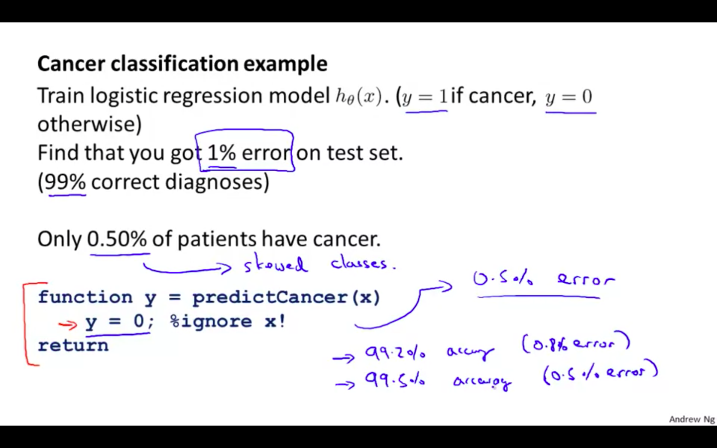
Cancer Classification Example
- When there are skewed classes in the dataset, then the classification evaluation metric is no longer efficient way to identify model’s accuracy.
-
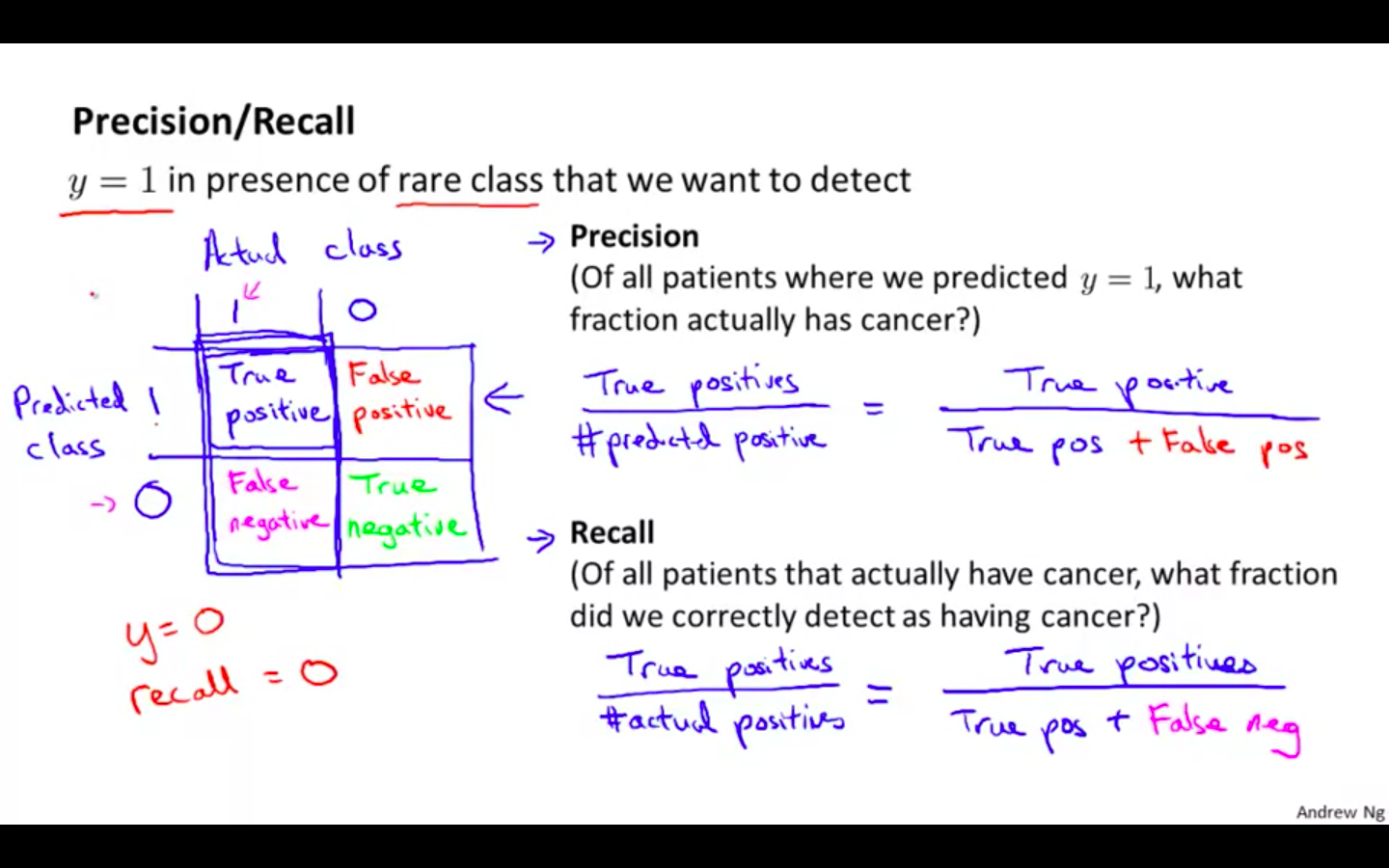
Precision / Recall
-
Precision is number of true positives divided by the num of predicted positives i.e True Positives + False Positives
-
Recall is number of true positives divided by the num of actual positives i.e True Positives + False Negatives
-
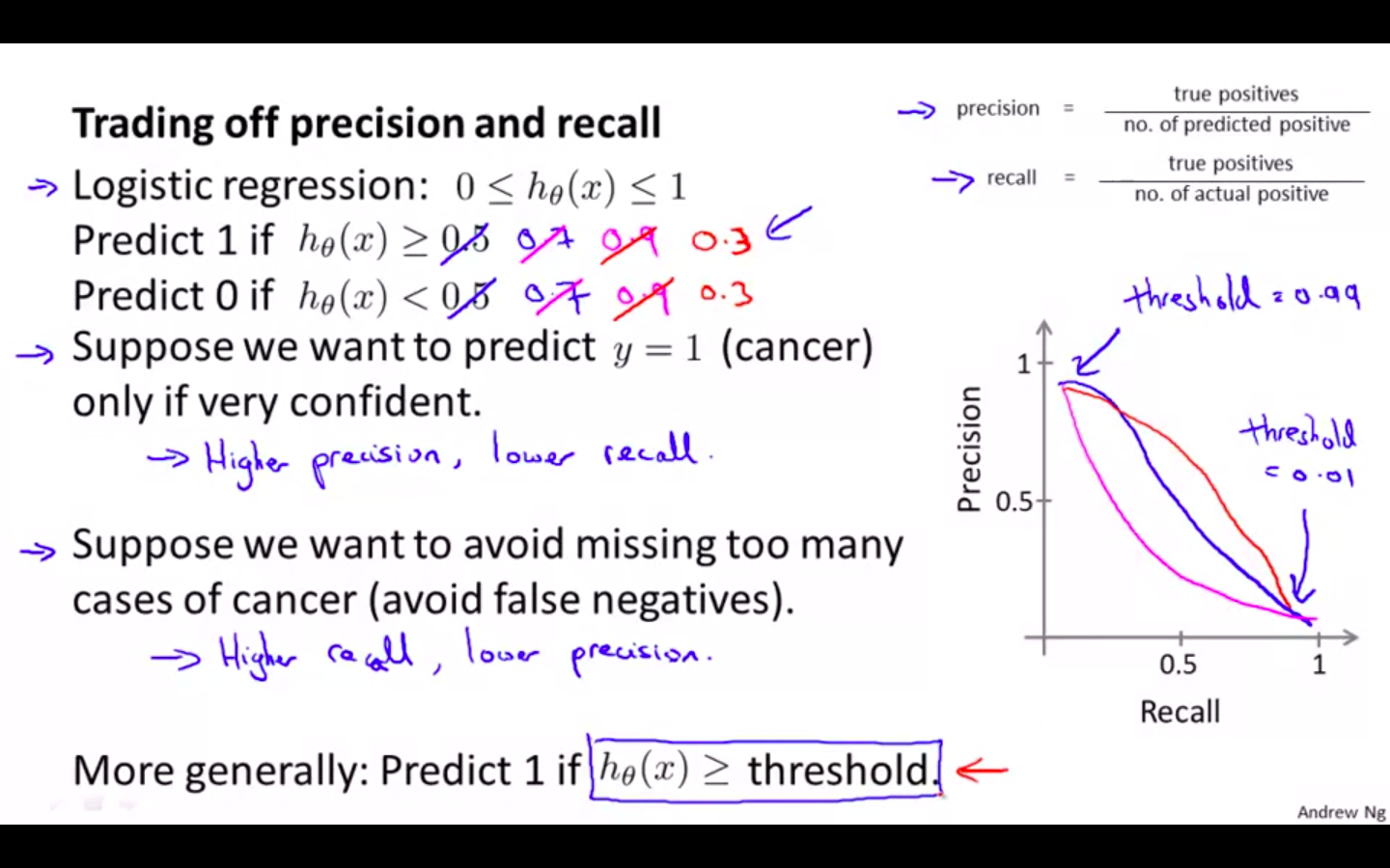
Trading Off Precision and Recall
-
Trade Off
-
If threshold is high then the precision will be high and recall would be low
-
If threshold is low then the precision will be low and recall would be high
-
-
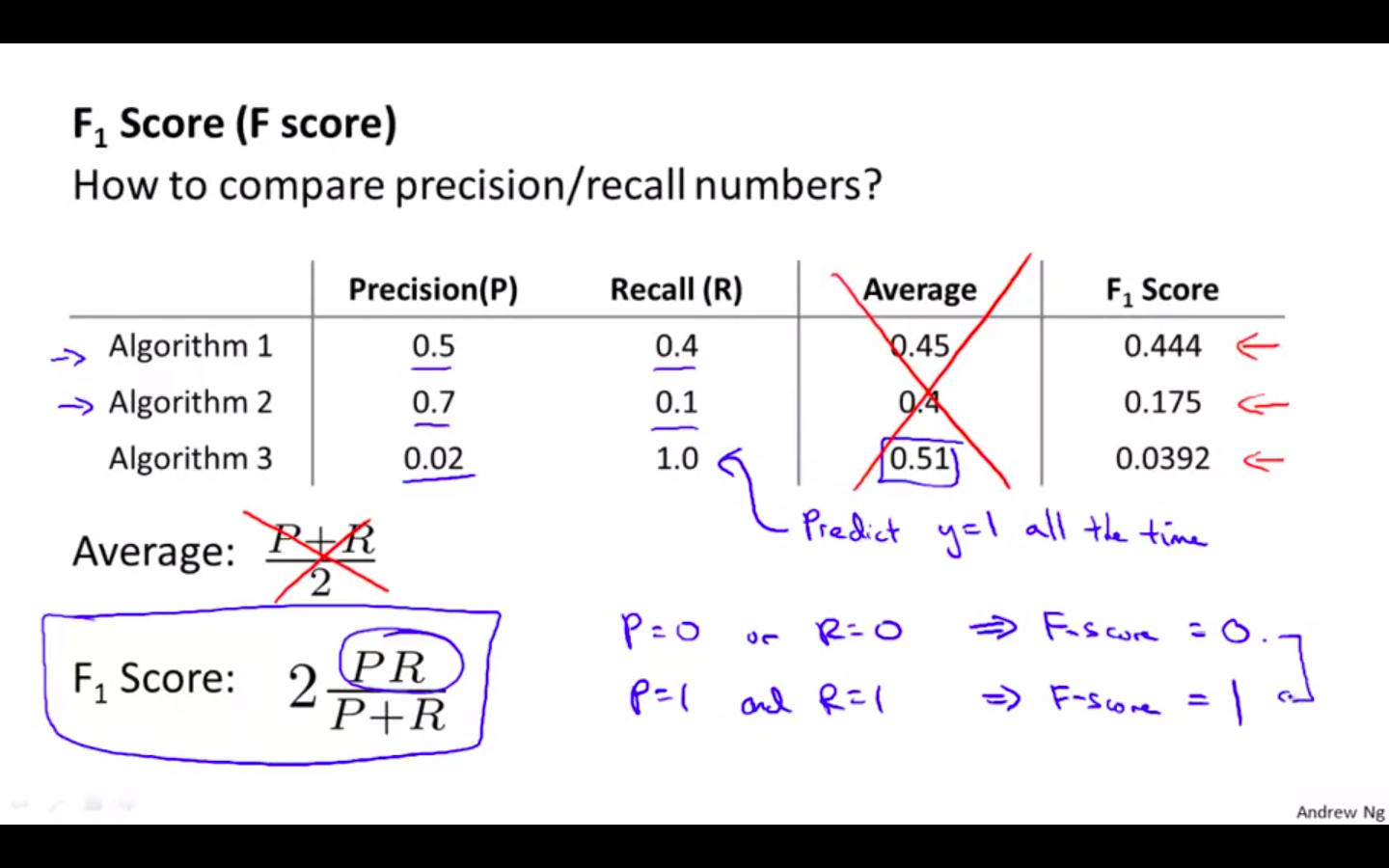
F Score
-
Numeric evaluation metric for the model’s with skewed data
-
$ F = 2 * PR / P + R $
-
P = 0 && R = 0 ⇒ F = 0
-
P = 1 && R = 1 ⇒ F = 1
-
Using Large Datasets
Data For Machine Learning
-
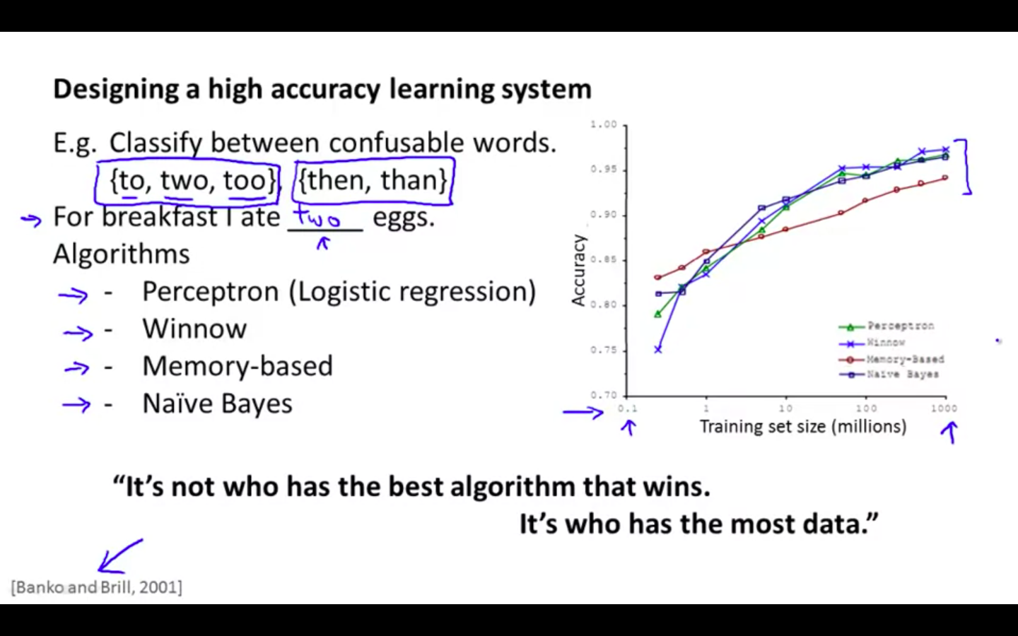
Research Paper
- Inferior algorithms can perform as well as superior algorithms when provided with lot of data
-
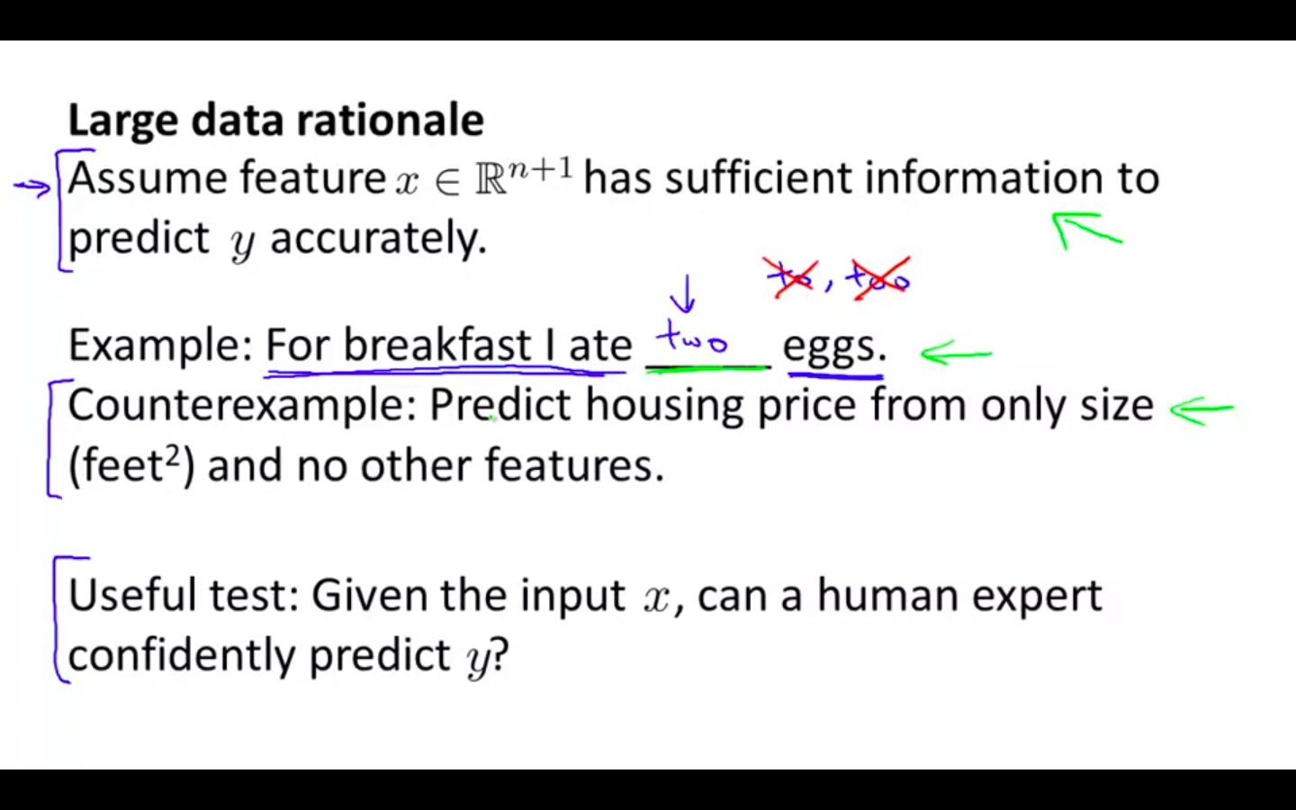
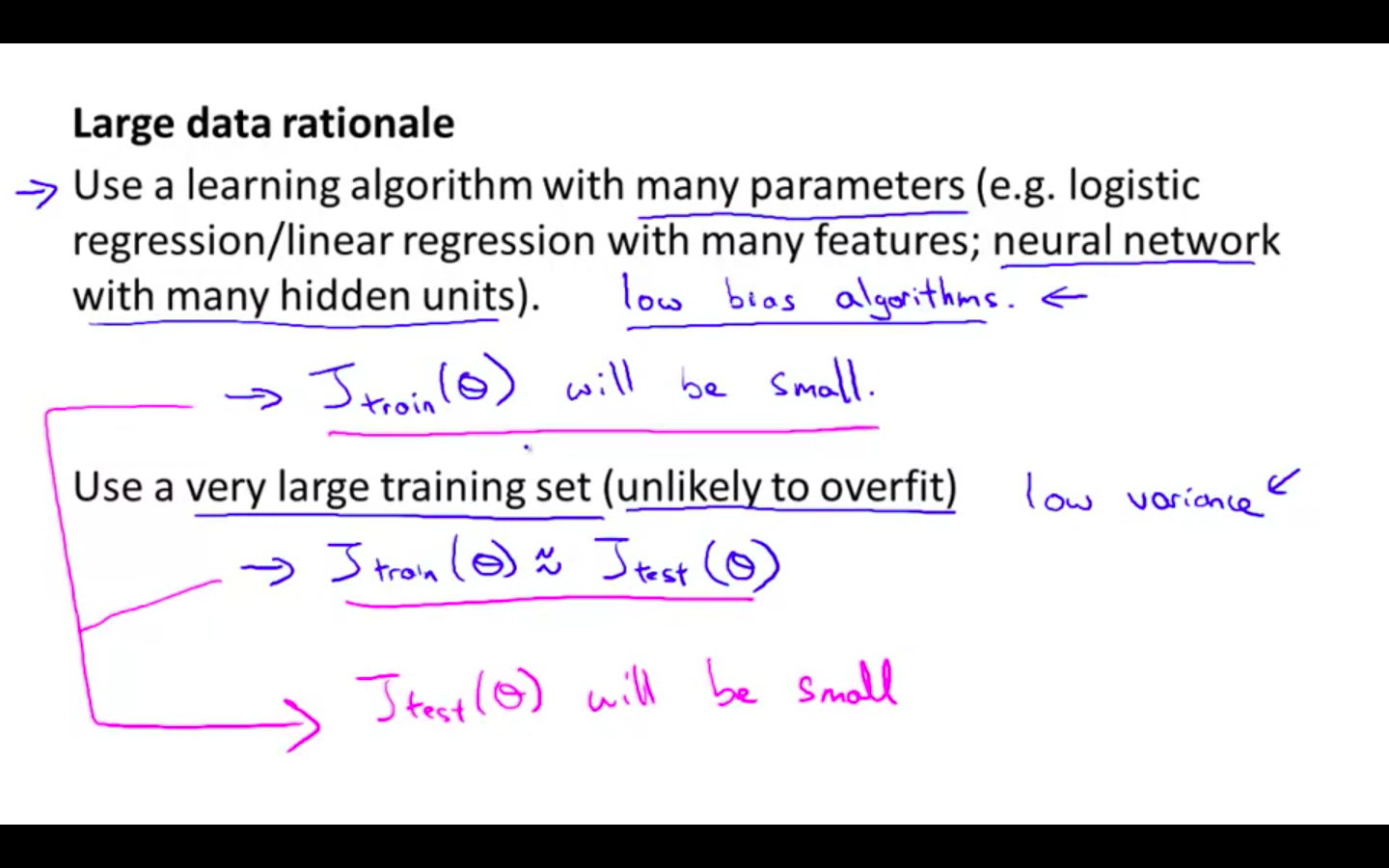
Large Data Rationale
-
Cases when large data is useful
-
Useful Test: Given the input x, can a human expert confidently predict y ?
-