Machine Learning By Andew Ng - Week 10

Gradient Descent with Large Datasets

Learning With Large Datasets

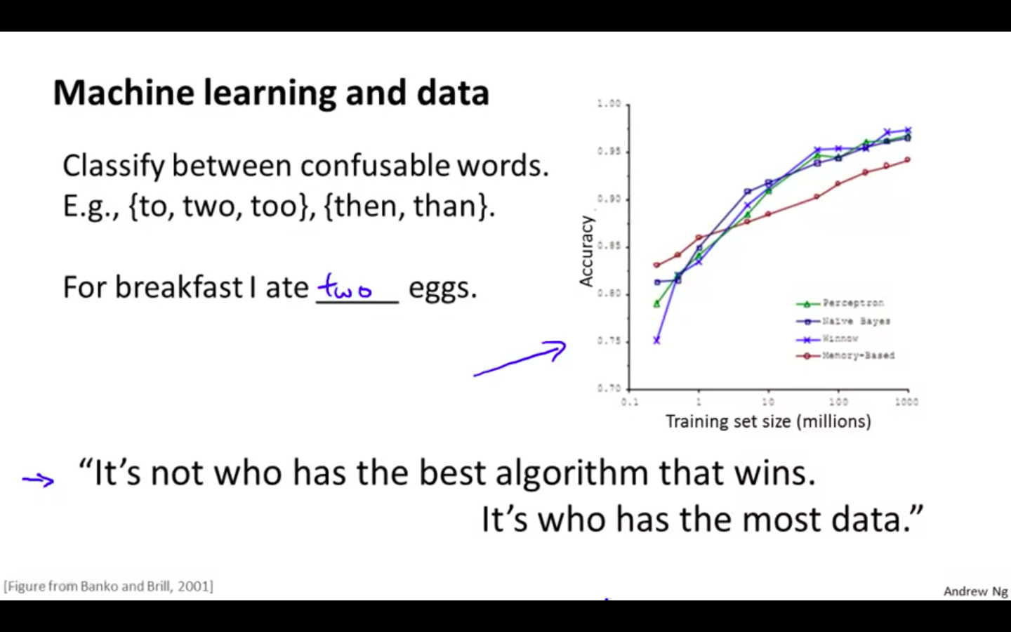
• Machine Learning and Data

  It’s not who has the best algorithm that wins. It’s who has the most data.

  

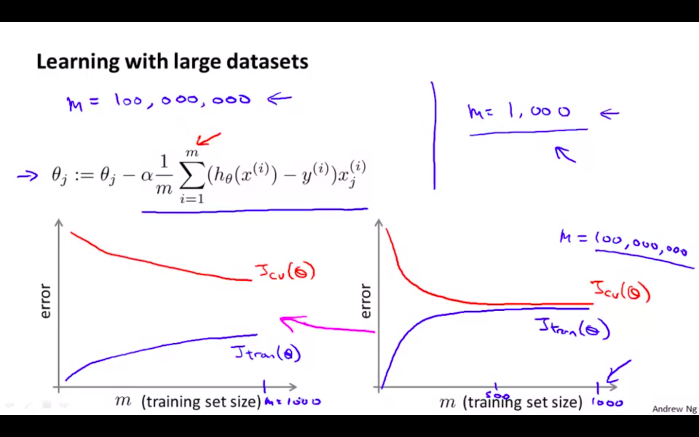
• Learning With Large Datasets

  • First choose m = 1000 and train the algorithm

  • Plot the learning curve, if it has high variance then more data feeding will be helpful

  • If the learning curve is high bias then more data feeding will not be helpful

  

Stochastic Gradient Descent

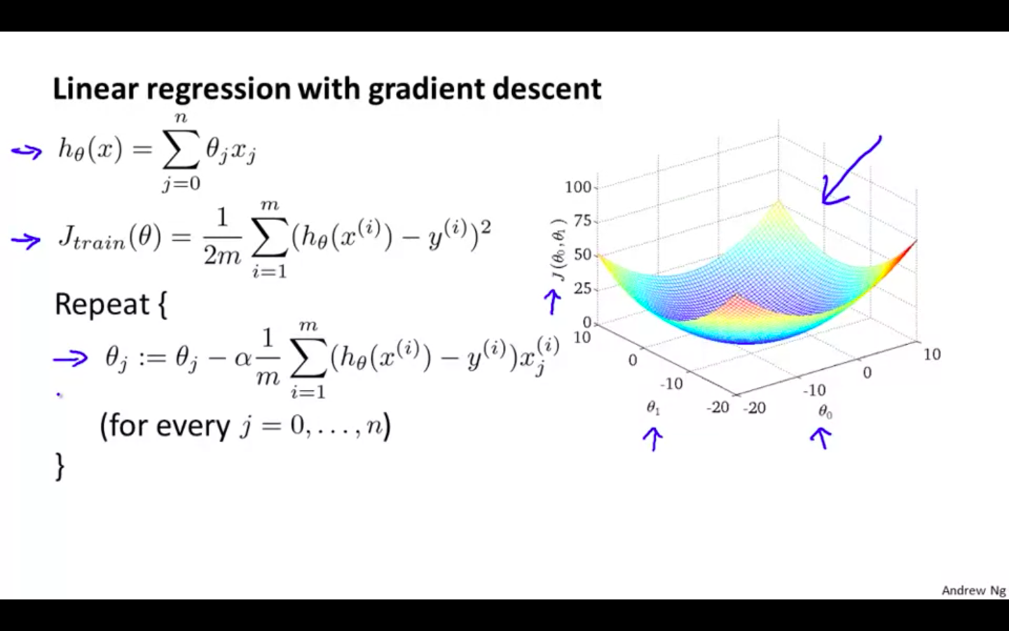
• Linear Regression with Gradient Descent

  • Recap

  

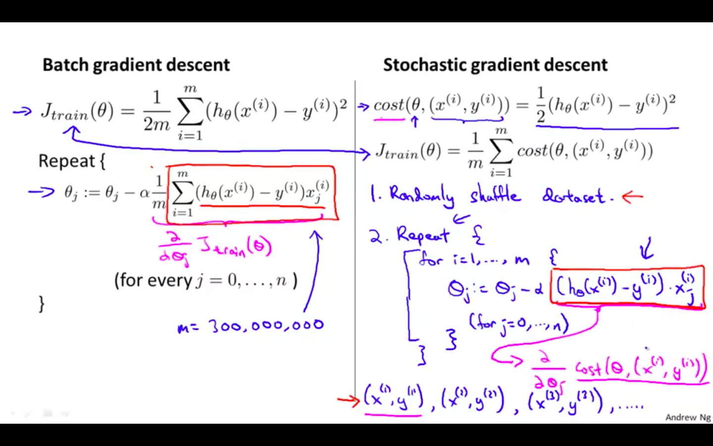
  • Previous from of gradient descent would iterate all the training examples and sum them to take one step of descent

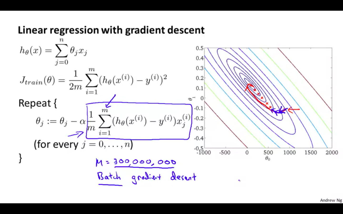
  • This causes problem when the training data is way too large, in hundreds of millions, then it gets computationally expensive to use that gradient descent

  • That is also called as “ Batch Gradient Descent “, because it uses all the training data

  

• Batch Gradient Descent vs Stochastic Gradient Descent

  

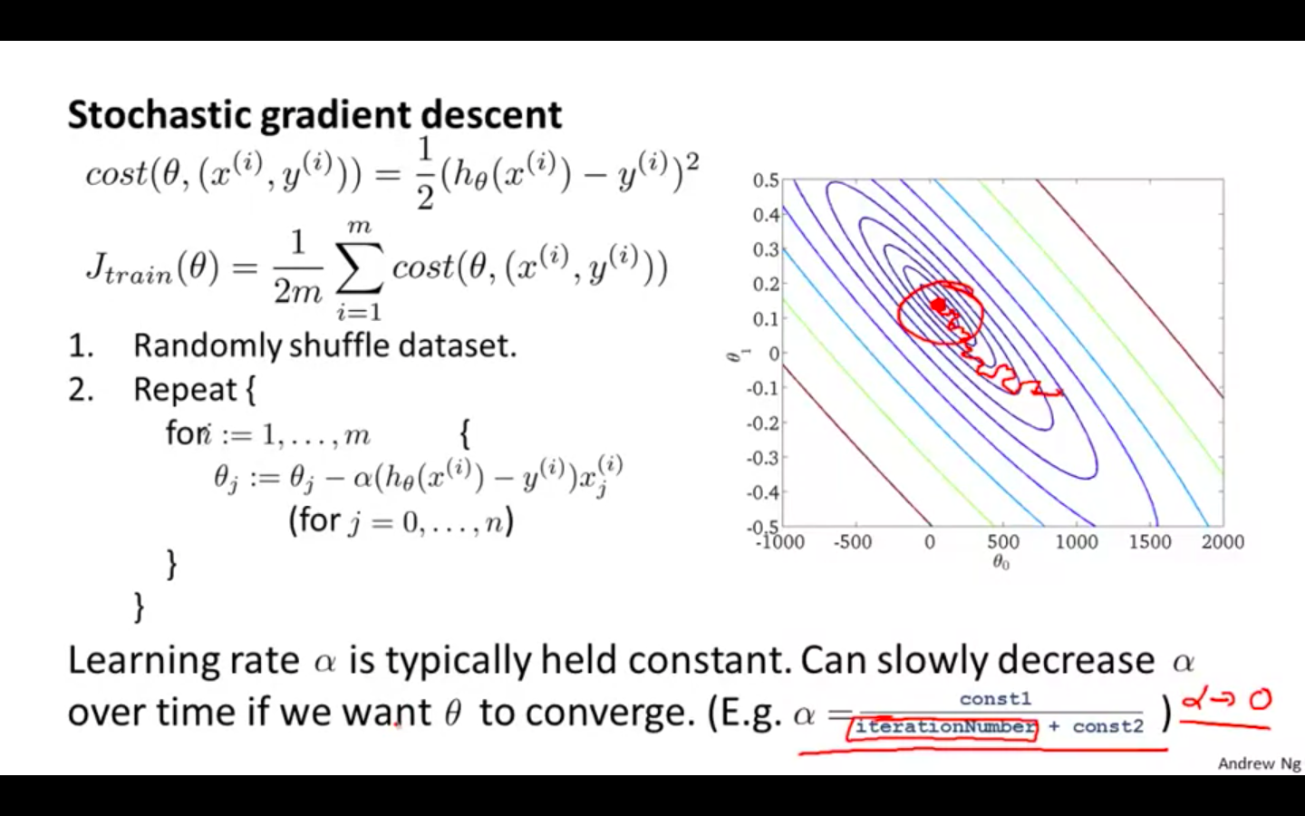
• Stochastic Gradient Descent

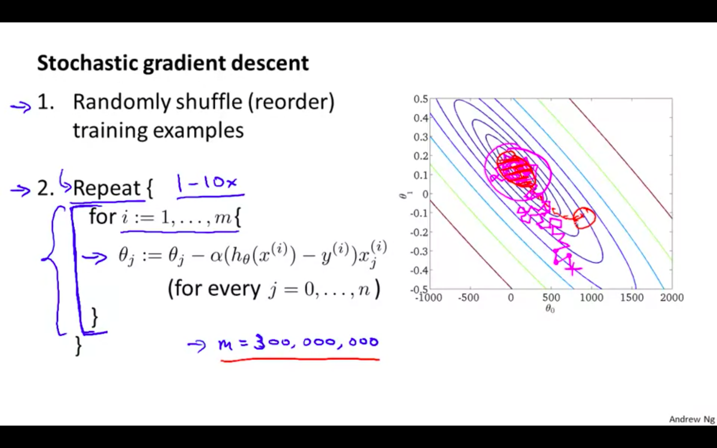
  • Randomly shuffle the training data

  • Repeat the descent using one single example at a time

  • Descent will not converge like the batch gradient descent, it will get to the area of the global minimum which is good for the hypothesis

  • This will not converge directly to the global minimum

  • Steps are in variation to each other and in whole picture, it is moving towards the global minimum

  

Mini-Batch Gradient Descent

• Comparison between different gradient descent

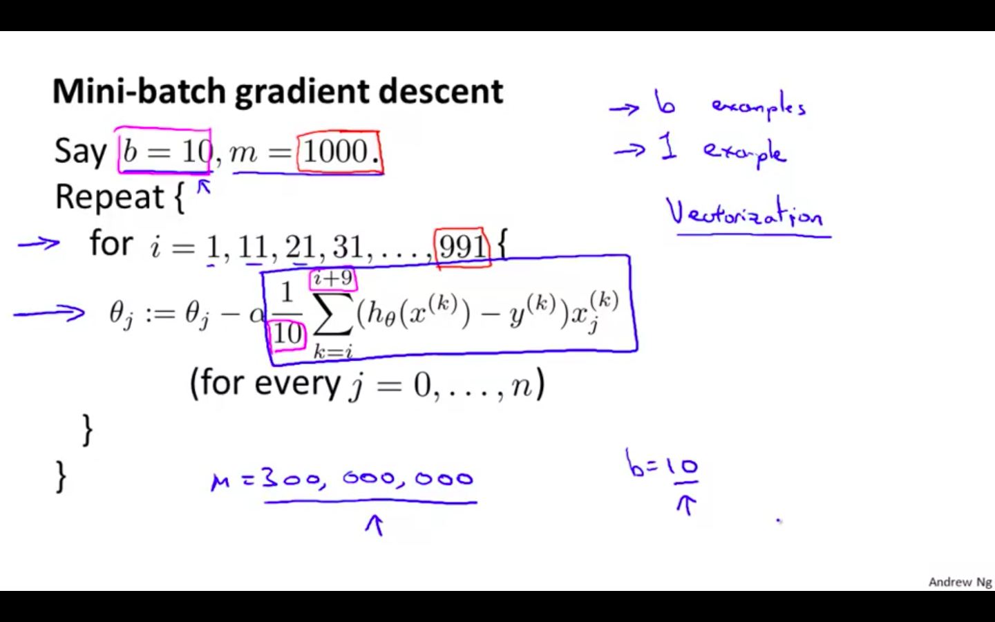
  • Batch Gradient Descent ⇒ Use all m examples in each iteration

  • Stochastic Gradient Descent ⇒ Use 1 example in each iteration

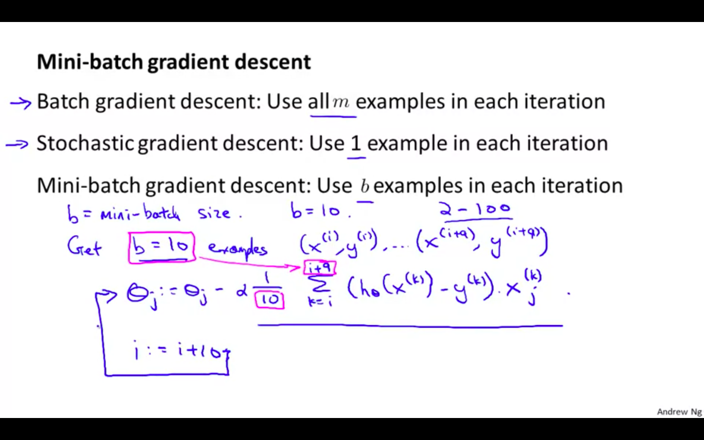
  • Mini-batch Gradient Descent ⇒ Use b examples in each iteration

  

• Mini-Batch Gradient Descent

  • Select a no. of examples for batch

  • Repeat the descent updates using the new batch

  • It is faster than the batch gradient descent

  • If vectorisation implemented efficiently it can be faster than the stochastic gradient descent, because of the parallelism used in operations

  

Stochastic Gradient Descent Convergence

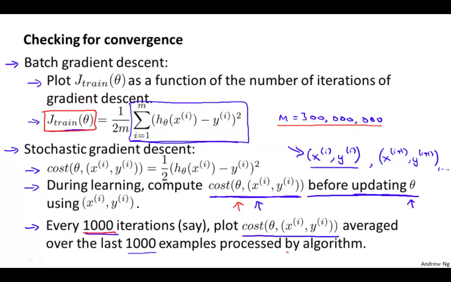
• Checking for Convergence

  • During learning compute cost function before updating parameter

  • Every 1000 iteration ( say ), plot cost function averaged over the last 1000 examples processed by algorithm

  

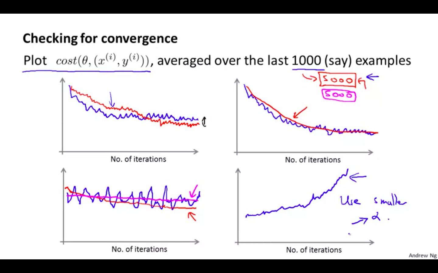
  • Examples

    • Using bigger number of training examples before ploting will give a smoother curve

    • If cost seems to increase increase, it means the algorithm has diverge.

      • Using smaller learning rate will solve the problem

    

• Tuning Learning Rate in Stochastic Gradient Descent

  • Learning rate alpha is typically held constant. Can slowly decrease alpha over time if we want theta to converge

    • alpha = const1 / iterationNumber + const2

  • Dynamic selection of learning rate can result in convergence of the algorithm

  • Small learning rate will result in not oscillating around the global minimum and to converge

  

Advanced Topics

Online Learning

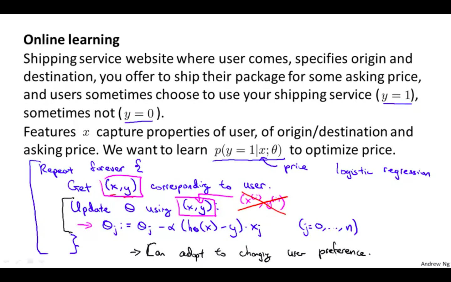
• Online Learning

  • Shipping service website where user comes, specifies origin and destination, you offer to ship their package for some asking price, and users sometimes choose to use your shopping service ( y =1 ), sometimes not ( y = 0 )

  • Features x capture properties of user, of origin / destination and asking price.

  • We want to learn p ( y = 1

    x ; theta ) to optimise price.

  • In online learning, there is no fixed training data

  • There is continuous stream data flowing which is used to train once and then the data is discarded

  • Online learning can adapt to changing user performance

  

• Examples

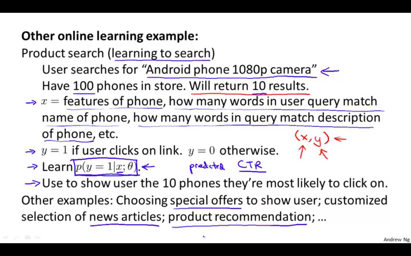
  • Product search ( learning to search )

    • User searches for “ Android phone 1080p camera “

    • Have 100 phones in store. Will return 10 results

    • x = features of phone, how many words in user query match name of phone, how many words in query match description of phone etc

    • y = 1 if user clicks on link. y = 0 otherwise

    • learn p ( y = 1

      x ; theta )

    • Use to show user the 10 phones they’re most likely to click on

  • Choosing special offers to show user

  • Customised selection of news articles

  • Product recommendation

  

Map Reduce and Data Parallelism

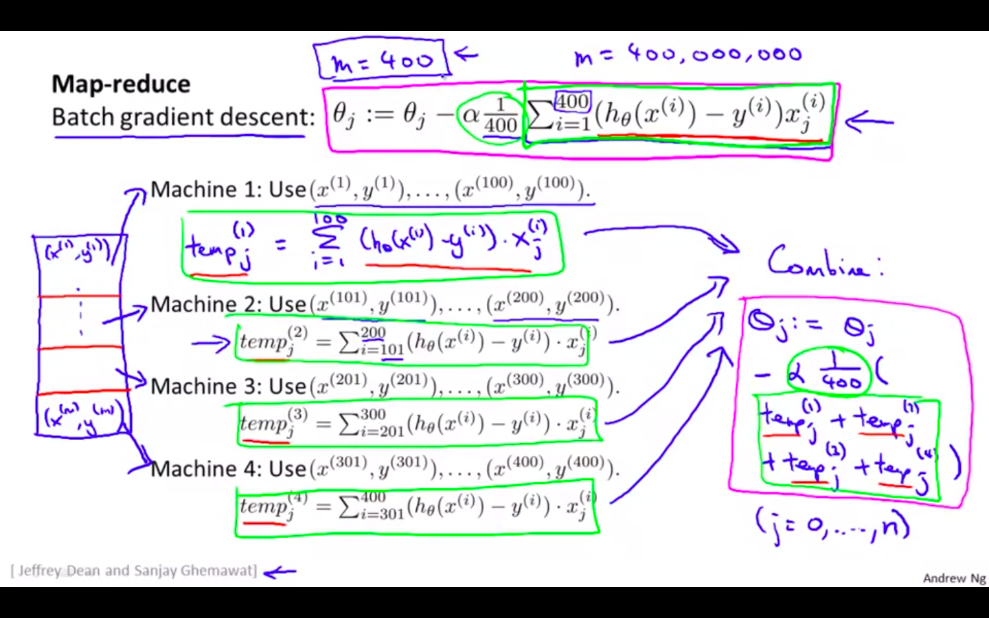
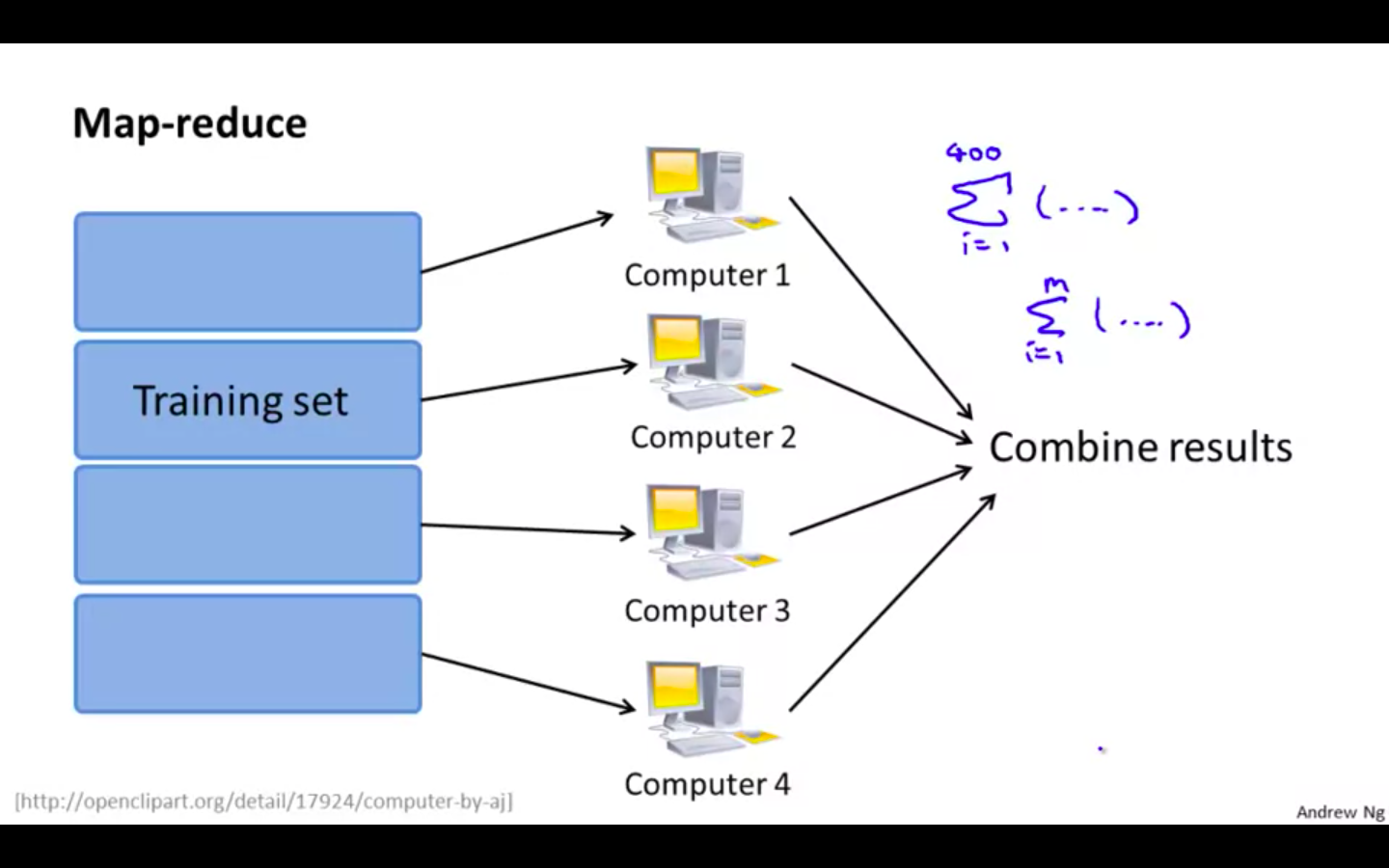
• Map Reduce

  • Dividing the training set into parts and computing them using different computers and then combining results from all computers

  • Network latency has to be considered

  

  • Concept

    • Workflow of Map Reduce

    

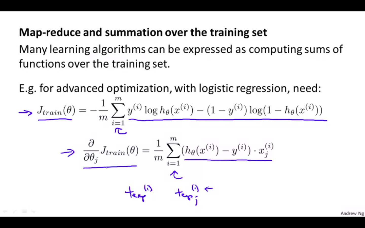
  • Map Reduce and summation over the training set

    • Many learning algorithms can be expressed as computing sums of functions over the training set

    

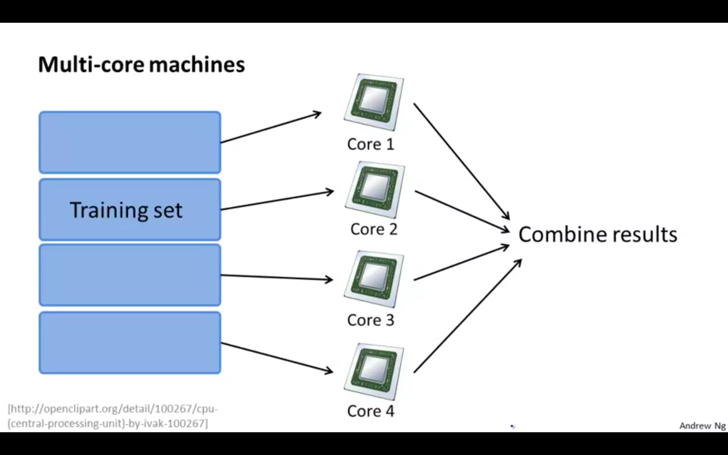
  • Multi Core Machines

    • It uses multiple cores in the machine to parallelise the operation

    • Factor of Network latency is diminished, because all the operations are performed in the same machine

    

Lecture Presentations